Assessing the impacts of mitigation and geoengineering intervention scenarios on Earth system dynamics and climatological variability with multimodal simulations
March 9, 2025
Abstract
Given a world increasingly dominated by climate extremes, modifying the Earth’s climate with large-scale geoengineering intervention is inevitable. However, geoengineering faces a conundrum: forecasting the consequences of climate intervention accurately in a system for which we have incomplete observations and an imperfect understanding. We evaluate the global response and potential implications of mitigation and intervention deployment by utilizing CRU TS4.08 observations, ERA5 reanalysis data, and CMIP6 scenario-based UKESM0-1-LL simulations. From 1950 to 2022, global weighted mean surface temperature (Tsurf) and total precipitation (P) rose by 1.37(:pm:)0.48 °C and 0.05(:pm:)0.57 mm day-1. Significant regional Tsurf anomalies and erratic interannual variability of P were revealed, with ranges from 7.63 °C in Greenland and northern Siberia to -2.38 °C in central Africa and 1.17 mm day-1 in southern Alaska to -1.20 mm day-1 in Colombia and east Africa. Collectively, mitigation and intervention simulations tended to overestimate the variability and magnitude of Tsurf and P, exhibiting substantial regional discrepancies and scenario-specific heterogeneity when estimating atmospheric methane concentration ([CH4]). Despite capturing significant departures in Tsurf, P, and [CH₄], replicating historical P teleconnections and spatial patterns of warming remained a challenge. These results underscore regional disparities with global implications, harkening the necessity to refine existing architectures while developing novel methods to evaluate the risks and feasibility of geoengineering intervention.
Introduction
State-of-the-art climate models failed to explain why global temperatures spiked in 2023, with a 0.2 °C divergence between expected and observed annual mean temperatures, suggesting that the world may be entering uncharted territory1. Climate change is accelerating while anthropogenic greenhouse gas (GHG) emissions continue to rise, risking the ability of the global community to achieve key climate stabilization targets2. For decades, climate models warned of linear atmospheric warming and nonlinear changes to the land surface. Despite this warning, global net emissions of anthropogenic greenhouse gases reached record levels over the last decade3. Current projections suggest that barring significant mitigation efforts, the cumulative concentration of greenhouse gases will likely eclipse the 1.5 °C climate stabilization threshold by 2035, a stark acceleration from previous forecasts4. If left unabated, there is a 67% likelihood that current emissions trends could exhaust the remaining carbon budget in less than a decade5.
These events drive an increasing demand for global solutions to mitigate climate change, and the deployment of geoengineering technologies appears increasingly inevitable6. Geoengineering – the deliberate large-scale intervention in the Earth system to manipulate specific biogeochemical processes or elements of the physical climate to counteract the impacts of climate change – presents an intricate problem: what strategies to implement and when to implement them. As the planet continues to warm and GHG emission reduction and carbon removal methods fall short of their goals, offsetting these growing climate impacts will likely require direct modifications5,7,86. According to the World Meteorological Organization (WMO), weather modifications to mitigate climate warming are currently operational, with approximately 50 countries and nine U.S. states deploying regional climate engineering projects without regulation via interstate provisioning, e.g., cloud seeding (i.e., rain enhancement)9. Recent geoengineering proposals seek to reduce global temperatures and carbon dioxide concentrations ([CO2]) to preindustrial levels10,11,12,13. Some methods involve offsetting climate change impacts by solar radiation management (SRM)14. SRM strategies involve the injection of sulfate aerosols into the stratosphere to achieve regional climate balance by reflecting sunlight to cool the planet15. Aside from the feedback repercussions of this approach (i.e., amplified ocean acidification), SRM strategies introduce significant uncertainties16,17. These uncertainties originate from the assumption of a uniform distribution of aerosols in both hemispheres; in reality, adopting SRM methods could precipitate an uneven spatiotemporal distribution of cooling effects across different latitudes and seasons with unknown secondary and tertiary consequences6,10. Stratospheric aerosol injection (SAI) remains a widely discussed SRM climate intervention mechanism for reducing Tsurf, though it may result in catastrophic side effects, including reduced productivity or global breadbasket collapse18,19,20,21,22,23,24. Alternative SRM proposals include deploying space reflectors and a space-based solar shield, thinning cirrus clouds, brightening marine clouds, and injecting ice particles 17 km above the Earth’s surface to facilitate stratospheric dehydration25,26,27,28. Cirrus cloud seeding involves injecting silver iodide into the lower atmosphere to facilitate precipitation formation, mimicking ice crystallinity while altering the geochemical properties of supercooled mixed-phase clouds29,30,31. Modeling studies integrating global circulation models (e.g., ECHAM6-HAM, CESM-CAM5) and scenario-specific forcing data explore the feasibility of cloud seeding strategies and associated impacts on radiative and climate response patterns, demonstrating a reduction in cirrus-induced radiative effect (− 0.8 to -1.8 Wm-2), a reduction in CO2-induced climate change (50–85%), and mixed effects and uncertainty for extreme precipitation events32.
The challenge for geoengineering deployment is that these decisions will occur under high uncertainty and incomplete information and invariably require estimating the impact of physical phenomena beyond the range of the current observational record, thus minimizing the effectiveness of data-driven forecasts. Machine learning, neural networks, and other data-driven approaches generate interpolated forecasts based on training datasets that span relevant spatial, temporal, and physical parameter ranges occupied by the input and prediction sets. Despite their promise, data-driven approaches to speculative scenarios may introduce additional risks and biases that emerge from their fundamental assumptions and disjointed standards of practice. Accordingly, the uninformed application of data-driven methods can manifest as unintended risks and outcomes that are difficult to detect or diagnose even under manual inspection by domain experts33,34. Such oversight may originate from failing to rigorously assess model performance with sufficient data while supporting interpretability, explainability, and transparency35.
How do we harness data and state-of-the-art tools to address the fundamental challenges associated with when and how to deploy geoengineering solutions? Given an incomplete observational record and an imperfect knowledge and understanding of the Earth system and related feedbacks, what is the optimal use of these techniques and tools to guide intervention strategies36? What are the potential risks and unintended consequences of these decisions? This study explores these questions using multimodal data processing and modeling frameworks to match these complex challenges. We propose leveraging reanalysis products and model simulations to help optimize mitigation logistics, bridge multiscale intervention challenges, summarize contingency scenarios, and support continuous monitoring infrastructure. We examine various mitigation and geoengineering strategies and their subsequent impacts on the Earth system by using historical estimates from the fifth-generation, land-specific, global atmospheric reanalysis data subset (i.e., ERA5) ) and a series of mitigation and intervention experiments supporting the Coupled Model Intercomparison Project, Phase 6 (i.e., CMIP6)37. Mitigation experiments are derived from the Carbon Dioxide Removal Model Intercomparison Project (i.e., CDRMIP), while geoengineering intervention experiments are derived from the Geoengineering Model Intercomparison Project (i.e., GeoMIP)38,39,40,41. By utilizing existing observational systems and nascent technology effectively, we can monitor and interpret the biogeochemical processes, synergistic relationships, and spatiotemporal variability governing the Earth system, observe how regional and global climate baselines are changing, and better understand how the Earth and land-atmospheric responses will respond to mitigation and intervention deployment42.
Results
ERA5 reanalysis
For retrospective analysis, we examined high-resolution surface variables, i.e., 2-meter surface temperature (Tsurf) and total precipitation, i.e., precipitation flux (P) derived from the ECMWF ERA5 Monthly-Averaged Climate Reanalysis dataset over a 73-year period (i.e., 1950–2022). These data products provide global physics-based data-driven land surface postprocessed monthly-resampled observations on a 31-km rectilinear latitude-longitude grid (i.e., Methods, S1). The results below illustrate mean departures computed from monthly weighted climatologies with temporal thresholding (Fig. 1).
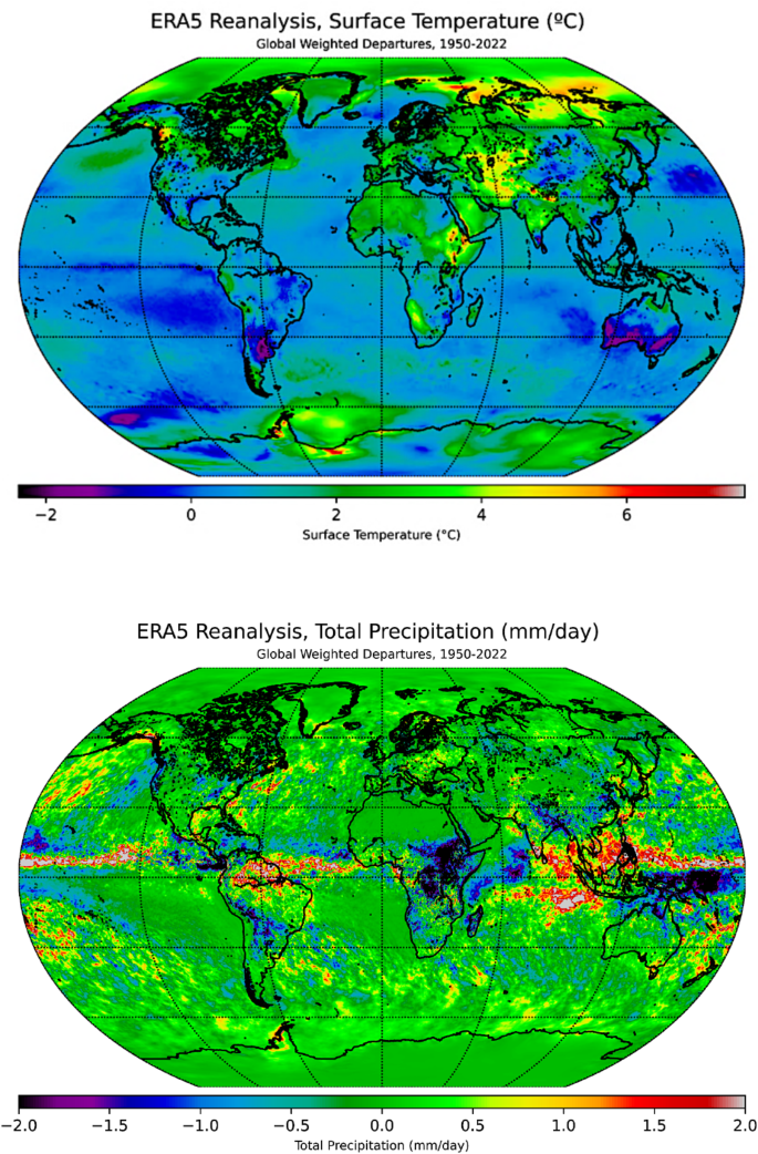
The monthly means of Tsurf and P were grouped by monthly time coordinates to compute global interannual weighted climatologies and departures from 1950–2022 (i.e., reference period: 1981–2010). Global departure variability is illustrated by both covariates, with subpanel time series illustrating anomalous dynamics in S1. The variabilities exhibit increasing Tsurf and P of 1.374±0.481ºC and 0.045±0.567 mm day−1, respectively. Climatologies, departures, and statistics are available in S1 and S9. The plots were generated with Python 3.9.18 and the various modules from the Matplotlib and Cartopy libraries43,44
Retrospectively, global mean Tsurf and P results from ERA5 reanalysis data indicate substantial climatological variability from the observed record during these 73 years. When resampled, these global and regional patterns remained intact; however, the statistical ranges varied; specifically, the regional Tsurf mean variability (i.e., departures) ranged between − 2.33-4.53(:^circ:)C, with increasing global mean Tsurf variability, i.e., 0.18(:pm:)0.59(:^circ:)C. Greenland, northern Siberia, the Horn of Africa, and the Antarctic coastline experienced elevated Tsurf as high as 7.63(:^circ:)C between 1950 and 2022, while central Africa, southern Australia, eastern Brazil, and northwestern Mexico observed notable reductions in Tsurf (-2.38(:^circ:)C); however, the global mean Tsurf steadily increased by 1.37(:pm:)0.48(:^circ:)C. During this period, regional Tsurf anomalies ranged from − 1.33(:^circ:)C across the Canadian Boreal and northern Siberia (e.g., Yamalo-Nenets Autonomous Okrug) to 1.19(:^circ:)C across the Arctic (e.g., Greenland, northwestern Alaska, Chukotka Autonomous Okrug), Antarctica, Uruguay, Angola, and southeastern China. Moreover, the global mean departures of Tsurf accounted for a significant reduction (-0.30 (:pm:)0.33(:^circ:)C).
In parallel, regions including southern Alaska (e.g., Chugach and Copper River), the northern coast of Norway, South America (e.g., western Ecuador, northern Brazil, Rio Grande do Sul, Uruguay), southern India, northwestern Indonesia, and Africa (e.g., Central Africa Republic, Democratic Republic of the Congo, Angola, South Africa) experienced increased P (1.17 mm day-1), South America (e.g., Colombia, Bolivia, Amazonas) and east Africa (e.g., Sudan, Ethiopia) experienced reductions in P (-1.20 mm day-1). The global mean P marginally increased by 0.05(:pm:)0.57 mm day-1. Furthermore, regional P departures indicate a decrease of -0.39 mm day-1 across the Amazon, Sahel, and Southeast Asia, while P anomalies exhibit nearly 0.13 mm day-1 in southeastern Africa (e.g., Zimbabwe, Mozambique). Reductions in the global mean P anomalies were computed, i.e., -0.03(:pm:)0.05 mm day-1. Similar to Tsurf variability after resampling, regional P departures ranged from − 5.11 to 5.55 mm day-1, with global mean P departures of 0.05(:pm:)0.57 mm day-1 (i.e., increasing precipitation, P > ET).
CMIP6 | CDRMIP simulations
For prognostication and simulation purposes, we simulated two CO2 removal (i.e., CDR) mitigation experiments with the UKESM0-1-LL model, including (1pctCO2-cdr) after the abrupt quadrupling of CO2, instantiate 1% CO2 reduction per year, i.e., 1pctCO2-cdr and (esm-1pct-brch-1000PgC) continuation of the zero-emission simulation branch from 1pctCO2-cdr after the 1000PgC cumulative emissions threshold was achieved, i.e., esm-1pct-brch-1000PgC. We employed additional historical and future controls on emissions reduction in the model simulations for retrospective and prognostic purposes. Concluding simulation analyses, we identify and compare discrepancies between these mitigation and intervention simulations relative to the resampled ERA5 observational record.
1pctCO2-cdr
During this idealized experiment, we used CO2 removal methods to reduce 4xCO2 baseline levels by 1% per year until the preindustrial control (PiC) was obtained and maintained, with increases in global weighted mean variability (i.e., detrending via annual climatology) of Tsurf (3.89(:pm:)2.62(:^circ:)C), P (0.17(:pm:)0.78 mm day-1), and [CH4] (0.01(:pm:)0.27 ppb) over the 1990–2149 time period (Fig. 2). Interestingly, the global weighted mean variability further condensed these trends to decreasing Tsurf and P (-1.91(:pm:)1.22(:^circ:)C, -0.26(:pm:)1.13 mm day-1), while [CH4] increased (0.03(:pm:)0.02 ppb).
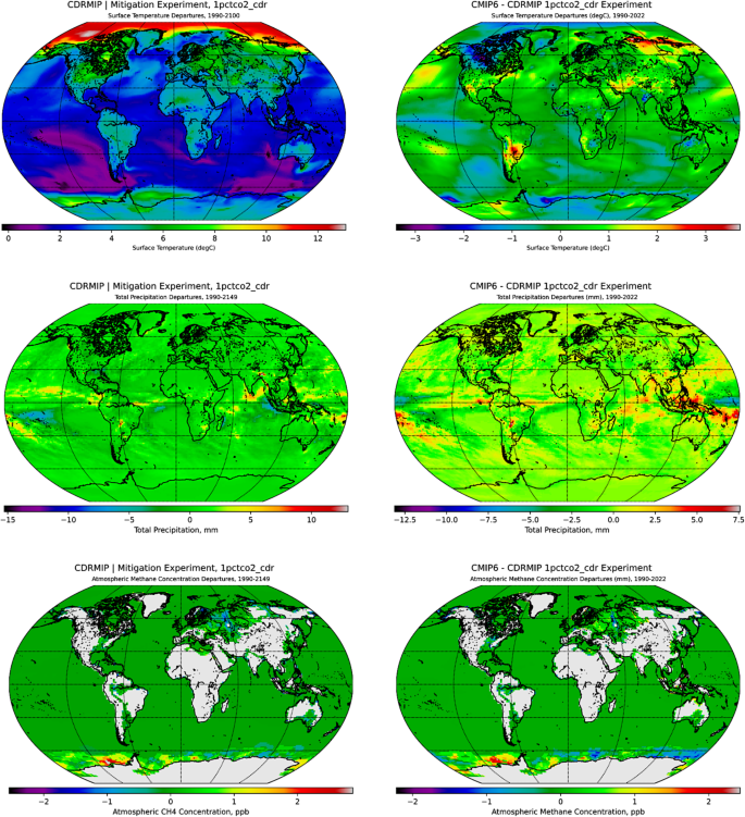
The first vertical panel above illustrates the weighted departures for annual periodicity of Tsurf ((:^circ:)C), P (mm day− 1), and [CH4] (ppb, 300-1,000 hPa) from the first CDRMIP experiment (i.e., 1pctCO2-cdr) simulated by UKESM1-0-LL. The second vertical panel expands on the departure variabilities (i.e., reference period: 1991–2020) constrained to the observational record (S8). Additional plots delineating on weighted and unweighted climatologies, departures, and temporal windows for ERA5 intercomparisons (i.e., 1pctCO2-cdr, 1990–2149 [1990–2022]) are contextualized in S2 and S8, with comprehensive statistics provided in S10. The plots were generated with Python 3.9.18 and the various modules from the Matplotlib and Cartopy libraries43,44.
The most compelling relationship with this first experiment is the clear indication of pronounced Arctic amplification and widespread warming (-0.25-13.08(:^circ:)C), with hotspots near Hudson Bay, the Bering Sea, Baffin Bay, eastern Europe, and the Middle East in addition, amplified [CH4] variability occurred along the Antarctic Peninsula coastline (-2.55-2.87 ppb), with pronounced warming surrounding Ellsworth Land, the Ross Ice Shelf, and north of Queen Maud Land. In contrast, large regions of the South Pacific Ocean and the Indian Ocean demonstrated clear indications of cooling, potentially driven by the deep-water formation, westerlies, and surface currents, i.e., westward wind drift from the Antarctic Circumpolar Current and the Peru Current and possibly catalyzed by the Northern Subpolar Gyre collapse, as indicated by the inactivity of P variability across the mid-latitudes. The most significant variability in P may be attributed to ocean-atmospheric equatorial interactions in the Arabian Sea (-12.23–9.06 mm day-1), Marshall Islands, and eastern Bolivia.
To differentiate regional patterns over this period, we examined the historical relationships between simulation outputs of Tsurf and P derived from this 1pctCO2-cdr experiment in alignment with the temporal windowing characterizing the ERA5 reanalysis observational record (i.e., 1990–2022, S10). Most significantly, these tri-decadal simulations predominantly overestimate global weighted Tsurf anomalies (6.88(:pm:)0.01ºC) and marginally underestimate global weighted P (-0.102(:pm:)0.003 mm day-1), with subsequent weighted mean departures for Tsurf and P (3.784(:pm:)2.004(:^circ:)C, 0.43(:pm:)0.91 mm day-1). Furthermore, Tsurf and P decreased (-0.01(:pm:)0.37ºC, -0.02(:pm:)0.89 mm day-1) while [CH4] increased (0.02(:pm:)0.25 ppb) over this period. Moreover, we examined global weighted departures and noted Tsurf and [CH4] increased (0.01(:pm:)0.72ºC, 0.03(:pm:)0.23 ppb) while P decreased (-0.09(:pm:)0.39 mm day-1) over this 33-year window.
esm-1pct-brch-1000PgC
For the next experiment, we emulated a zero-emissions scenario from the previous 1pctCO2-cdr experiment, with [CO2] removal continuing beyond achieving the 1000 Pg threshold for cumulative emissions from 1950 to 2149. Over 200 years of continued [CO2] reduction, the global mean climatologies characterizing all three covariates increased, with Tsurf increasing 0.06(:pm:)0.35ºC, P increasing by 0.003(:pm:)0.331 mm day-1 and elevating [CH4] by 0.001(:pm:)0.169 ppb (Fig. 3). Alternatively, the global weighted mean variability exhibited by all three covariates decreased, with Tsurf departures ranging from − 5.45-4.85(:^circ:)C, P variability from − 5.40 to 5.22 mm day-1, and [CH4] departures ranging from − 1.73 to 2.52 ppb. This coupled relationship is further illustrated by the mean of the global weighted mean variability computed for each covariate: -0.17(:pm:)0.83(:^circ:)C, -0.01(:pm:)0.67 mm day-1, and − 0.001(:pm:)0.188 ppb, respectively.
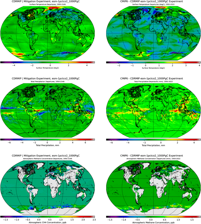
The first vertical panel above illustrates the weighted departures for the annual periodicity of Tsurf ((:^circ:)C), P (mm day− 1), and [CH4] (ppb, 300-1,000 hPa) from the second CDRMIP experiment (i.e., esm-1pct-brch-1000PgC) simulated by UKESM1-0-LL. The second vertical panel expands on departure variabilities (i.e., reference period: 1991–2020) constrained to the observational record (S8). Additional plots delineating weighted and unweighted climatologies, departures, and temporal windows for intercomparisons (i.e., esm-1pct-brch-1000PgC, 1950–2149 [1950–2022]) are provided in S3 and S8, with comprehensive statistics located in S10. The plots were generated with Python 3.9.18 and the various modules from the Matplotlib and Cartopy libraries43,44.
We evaluated regional changes in mean covariability over time. The results suggest that warming is less pronounced and more stochastic globally, with increasing Tsurf variability occurring west of the Antarctic Peninsula and distributed across the Norwegian and Greenland Seas, extending into the Arctic Ocean (4.85(:^circ:)C). Increasing P departures and cluster densities were localized to equatorial regions of eastern Brazil, French Polynesia, Arabian Sea and Bay of Bengal, northern Vietnam, and east of the Coral Sea (7.47Â mm day-1). In addition, we observed increased variability of the [CH4] mean in the Komi Republic, isolated anomalies occurred near the Northwestern Passages, and relatively minor plumes developed near the Amundsen Sea coastline and between Wilkes and Victoria Land (2.52 ppb). In contrast, the regional mean variability in Tsurf decreased near the Kara and Laptev Seas, the Canadian boreal zone, and the Amery Ice Shelf in Antarctica (-5.45(:^circ:)C), while [CH4] departures decreased near the Bellingshausen Sea and off the coast of Eastern Antarctica (-1.73 ppb). Bands of P variability are distributed across equatorial Oceania near the Hawaiian Islands, off the coast of eastern Brazil (i.e., Pernambuco), and north of the Solomon Islands and Papua New Guinea (-7.38Â mm day-1).
Historical simulations from the esm-1pct-brch-1000PgC experiment were compared with the ERA5 observational record, ensuring temporal alignment over 1950–2022, wherein zero-emissions were emulated from the 1pctCO2-cdr run after achieving the cumulative emissions 1000 Pg threshold (S3). During the intercomparison, simulations overestimate the global weighted mean of Tsurf (2.88(:pm:)0.07ºC) and underestimate the P (-0.101(:pm:)0.003 mm day-1). In addition, global climatologies and weighted mean variabilities were computed, resulting in the following climatologies: Tsurf (-0.03(:pm:)0.30(:^circ:)C, with ranges between − 3.20-3.44(:^circ:)C), P (0.001(:pm:)0.330 mm day-1, ranging from − 3.62 to 2.37 mm day-1), and [CH4] (0.01(:pm:)0.16 ppb, with ranges of -1.63-1.81 ppb). We computed global weighted mean departures, with simulations tending to overestimate Tsurf (0.05(:pm:)0.61ºC) and [CH4] (0.01(:pm:)0.17 ppb) while narrowly underestimating P (-0.0003(:pm:)0.5830 mm day-1).
CMIP6 | geomip simulations
Similarly, we conducted model simulations with the UKESM0-1-LL Earth system model components (e.g., aerosol, atmospheric, oceanic general circulation models, biogeochemical models) across four retrospective and prognostic geoengineering experiments. These four experiments and their corresponding climatological and departure variabilities – Tsurf, P, and [CH4] anomalies, differ from the long-term global climatological mean. These experiments included (G1) an abrupt quadrupling of CO2 while simultaneously integrating solar irradiance reduction, i.e., solar dimming (i.e., G1); (G6Solar) high-to-medium solar net forcing reduction from SSP585 to SSP245 (i.e., G6Solar); (G6Sulfur) stratospheric sulfate aerosol injection to reduce the net radiative forcing from SSP585 to SSP245 (i.e., G6Sulfur); and (2d) cirrus cloud seeding to minimize the net radiative forcing from SSP585 by 1 Wm[-2 (i.e., G7Cirrus).
G1
The first intervention experiment simulated the instantaneous quadrupling of atmospheric CO2 concentration while simultaneously deploying solar irradiance reduction (i.e., dimming) strategies to establish a historical baseline. The results in Fig. 4 illustrate global Tsurf, P, and [CH4] weighted mean variability from 1850 to 1949, ranging between − 6.87-4.38(:^circ:)C, -5.80–8.14 mm day-1, and − 0.004-2.200 ppb, respectively. The global climatological mean of Tsurf, P, and [CH4] remained relatively stable, with Tsurf and P decreasing from − 0.01(:pm:)0.47(:^circ:)C and − 0.01(:pm:)0.32 mm day-1 while [CH4] increased over 100 years, i.e., 0.003(:pm:)0.180 ppb. This homeostatic behavior demonstrates a relatively balanced net radiation budget in response to reducing the solar constant by offsetting longwave radiative impacts with fast radiative responses and reducing shortwave radiation via stratospheric adjustments.
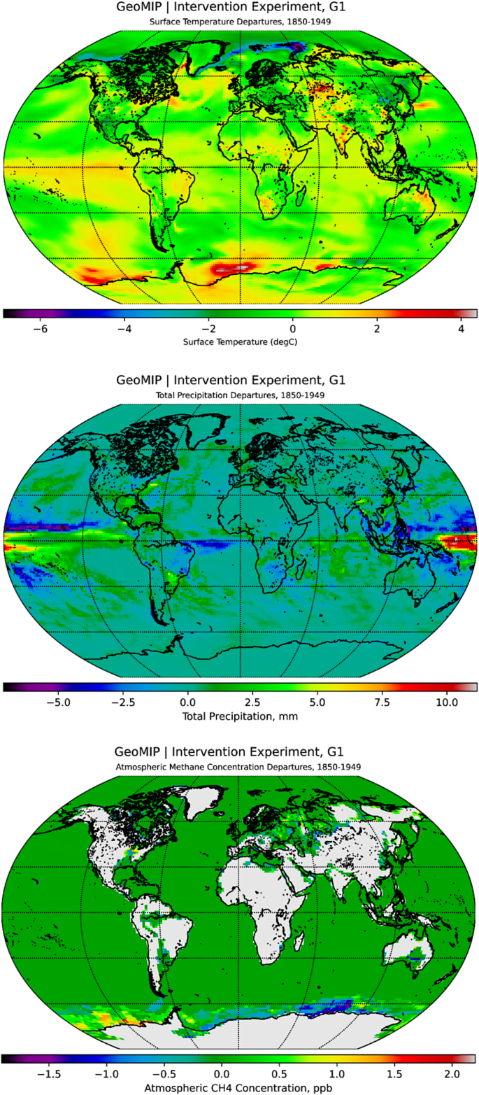
The panel above illustrates the weighted mean departures for Tsurf (°C), P (mm day− 1), and subtropospheric multilevel mean of [CH4] (ppb, 300-1,000 hPa) from the first GeoMIP experiment (i.e., G1) simulated by UKESM1-0-LL over the course of 100 years (i.e., 1850–1949). Additional plots delineating weighted and unweighted climatologies and departures are contextualized in S4 and S8, with comprehensive statistics provided in S10. The plots were generated with Python 3.9.18 and the various modules from the Matplotlib and Cartopy libraries43,44.
From a regional perspective, the global Tsurf mean variability increased from 1850–1949 (0.10(:pm:)0.85(:^circ:)C), with increased Tsurf departures displayed in the Middle East, northern Australia, Shandong, Sendai Bay, and several other Antarctic ice shelves including the Ronne Ice Shelf, Ross Ice Shelf, and Amery Ice Shelf, all demonstrating increased warming trends and pronounced ‘hotspot’ activity and variability (4.38(:^circ:)C). However, significant reductions in Tsurf variability were indicated primarily across the Chukchi and Beaufort Seas, as was the ‘mirroring’ of the Norwegian Atlantic Current period of the Atlantic Meridional Overturning Circulation near divergence in the Iceland Basin (0.15(:^circ:)C). Over 100 years, the P variability increased less steadily, with a total incremental P mean equivalent to 0.02(:pm:)0.81 mm day-1 across regional surfaces. Examining the regional patterns of global P mean departures, Micronesia, Uruguay, and Bangladesh experienced the highest magnitude relative to significant drying in Southeast Asia and eastern Brazil (-1.91–8.14 mm day-1).
To inform baselines with carbon flux data from G1 simulations, the historical evolution of the global mean [CH4] experienced abrupt pulses of increasing emissions yet maintained a marginal net sink progressively from 1850 to 1949, terminating with a net concentration difference of -0.001(:pm:)0.206 ppb. High concentrations of atmospheric carbon aggregated across Scandinavia, northwestern Siberia, and the coastline west of the Antarctic Peninsula near the Ross Ice Shelf and the Amundsen Sea (2.20 ppb), with noticeable opposing reductions in global [CH4] variability occurring along the eastern coast of Antarctica, emanating northeasterly from the Amery Ice Shelf into the Indian Ocean (-1.91 ppb). We did not conduct intercomparisons between resampled ERA5 reanalysis data and G1 simulations due to the temporal misalignment, i.e., ERA5 (1950–2022) v. G1 (1850–1949). However, after detrending G1 climatology to compute global mean departures from 1850 to 1949, Tsurf and P departures decreased from 1950 to 2022 relative to 1850–1949 (-0.24(:pm:)0.0.33(:^circ:)C, -0.17(:pm:)0.77 mm day-1), with ranges of -2.97-4.62(:^circ:)C and − 8.60–2.26 mm day-1, respectively.
G6Solar
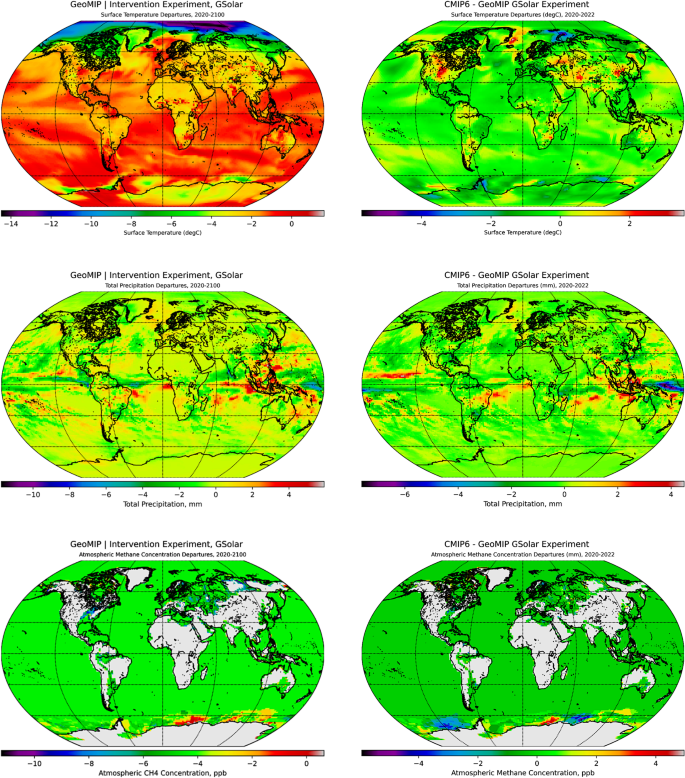
The second geoengineering experiment simulated high-to-medium solar forcing reduction efforts via solar irradiance curtailment (i.e., SSP585 to SSP245, 2020–2100). The radiative transfer dynamics evolve in response to the model’s instantiated variables, forcings, drivers, and parameterization. In essence, this experiment illustrates how solar geoengineering facilitates cooling effects, and the resulting maps and metrics demonstrate its utility and veracity for exploration and deployment. The global weighted climatological means for Tsurf, P, and [CH4] increased marginally from 2020 to 2100 (Fig. 5), ranging from − 1.15–6.59ºC (1.28(:pm:)1.26ºC), -2.62–5.26 mm day-1 (0.05(:pm:)0.35 mm day-1), and − 4.61–7.12 ppb (1.58(:pm:)1.08 ppb). The weighted mean variability of global Tsurf and P from 2020 to 2100 ranged between − 14.48-1.62(:^circ:)C, -10.52–3.92 mm day-1, and − 11.22–0.64 ppb, with a reduction in the global mean variability for Tsurf, P, and [CH4] indicated by -2.55(:pm:)2.61(:^circ:)C, -0.08(:pm:)0.61 mm day-1, and − 4.37(:pm:)0.62 ppb, respectively.
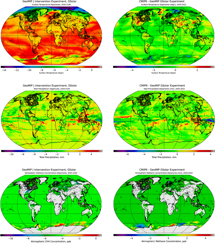
The first vertical panel above illustrates weighted mean departures for Tsurf (°C), P (mm day− 1), and subtropospheric multilevel mean of [CH4] (ppb, 300-1,000 hPa) from the second GeoMIP experiment (i.e., G6Solar) simulated by UKESM1-0-LL.The second vertical panel expands on the departure variabilities (i.e., reference period: 1991–2020) constrained to the observational record (S8). Additional plots delineating on weighted and unweighted climatologies, departures, and temporal windowing for ERA5 intercomparisons (i.e., G6Solar, 2020–2022 [2020–2100]) are provided in S5 and S8, with comprehensive statistics located in S10. The plots were generated with Python 3.9.18 and the various modules from the Matplotlib and Cartopy libraries43,44.
According to model simulations from this experiment, several regions exhibit hotspots for elevated Tsurf and [CH4] departures from planetary homeostasis, i.e., the climatological norm. These hotspots include Tsurf anomalies in northern and southeastern Brazil, the northern coastlines of Nunavut, the western coast of Baffin Bay, eastern Europe, northern Siberia, south Australia, Gujarat, and Indonesia. In addition to the clear equatorial gravitation for precipitation patterns, Uruguay exhibits periods of extended precipitation consistency. Alternatively, this intervention strategy introduces the concept of ‘cooling’ down the Earth: some spatial patterns of change emerge as ‘cold spots’ indicated by these results. In particular, these departures illustrate how the climate changes and moves away from past climatological norms. Although mostly constrained to open water at high latitudes, some cold spots include regions in the Bering and Barents Seas, Hudson Bay, and extending westward into the Greenland and Norwegian Seas.
Abiotic simulations predominately underestimate the global weighted mean variability of Tsurf (-0.17(:pm:)0.60ºC), P ( -0.01(:pm:)0.65 mm day-1), and [CH4] (-0.14(:pm:)0.56 ppb). We examined the resulting global mean temporal differences and variabilities between historical observations from resampled ERA5 reanalysis data and G6Solar simulations (i.e., 2020–2022). During ERA5 and G6Solar model intercomparisons of Tsurf and P from 2020 to 2022, the global weighted mean of mean differencing and standardized metrics were computed by spatially weighting the anomalies (i.e., weighted), removing climatological trends (i.e., unweighted), and applying a global mean operation across each observation and prediction originating from reanalysis data or simulation outputs (S3). Simulations from 2020 to 2022 indicated overestimations of Tsurf on the order of 0.02(:pm:)0.06ºC and underestimations of P variability by -0.102(:pm:)0.001 mm day-1. Interestingly, from 2020 to 2022, these upward-trending patterns of global mean Tsurf and P variability were observed and analyzed with respect to the overestimation of magnitudes. Furthermore, precipitation demonstrates intrinsic dynamic shifts in regime45; consequently, temporal subsetting permitted the isolation of trends for validation and sensitivity analyses. From 2020 to 2021, global weighted mean variability differencing of Tsurf and P from G6Solar simulations and ERA5 were overestimated (1.98(:pm:)0.03ºC, 0.865(:pm:)0.004 mm day-1) while both covariates subsequently overestimated across the 2021–2022 period, i.e., differencing resulted in Tsurf and P mean variability of 2.03(:pm:)0.08ºC and 0.88(:pm:)0.03 mm day-1, respectively, yielding net overestimations in Tsurf and P over this three-year validation window.
G6Sulfur
Stratospheric aerosol injection is simulated in this experiment (i.e., 2020–2100) to demonstrate the variability of forcing mechanisms and consequential impacts on the Earth system. Steady increases in the global mean climatologies of Tsurf, P, and [CH4] are represented by ranges of -1.05-6.41ºC (1.35(:pm:)1.30ºC), -2.22–3.13 mm day-1 (0.03(:pm:)0.33 mm day-1), and − 4.43–6.38 ppb (1.37(:pm:)1.18 ppb), respectively, until the end of the century (Fig. 6). Interestingly, all three covariates collectively experience reductions in global weighted mean variabilities, i.e., departures between the bounds of 2020 and 2100 (-2.70(:pm:)2.64ºC, -0.06(:pm:)0.65 mm day-1, and − 4.63(:pm:)0.99 ppb), illustrating persistent reductions in global mean Tsurf and [CH4] mean concentration. However, erratic oscillations prompt marginal reductions in P. Additional marked increases in the global weighted mean variability for P across eastern Brazil – from Bahia to São Paulo – and Tsurf and [CH4] anomalies near the Ross and Amery Ice Shelf.
The first vertical panel above illustrates weighted mean departures for Tsurf (°C), P (mm day− 1), and subtropospheric multilevel mean of [CH4] (ppb, 300-1,000 hPa) from the third GeoMIP experiment (i.e., G6Sulfur) simulated by UKESM1-0-LL. The second vertical panel expands on departure variabilities (i.e., reference period: 1991–2020) constrained to the observational record (S8). Additional plots delineating on weighted and unweighted climatologies, departures, and temporal windows for ERA5 intercomparisons (i.e., G6Sulfur, 2020–2022 [2020–2100]) are contextualized in S6 and S8, with comprehensive statistics provided in S10. The plots were generated with Python 3.9.18 and the various modules from the Matplotlib and Cartopy libraries43,44.
A comparison of ERA5 reanalysis data with historical simulations of SAI reveals a marked uptick in global mean Tsurf prior to climatological detrending, i.e., the increased warming trend is more explicit, suggesting that potential feedback interactions manifest and contribute to amplified overestimations of water cycle covariates, notably during the shoulder or transition seasons. Contemporary and CMIP6-derived simulation projections overestimate the magnitudes of some of these marginal/fringe oscillations, with future predictions (i.e., 2023–2100) of high-to-medium reduction (i.e., SSP585 to SSP245) via SAI demonstrating an even greater propensity to overestimate these covariates with large margins of magnitude differences. Therefore, temporal alignment with the observational record from ERA5 reanalysis during 2020–2022 allows observation-driven data and simulation output intercomparison to identify any correlations, relationships, or behaviors that manifest and contribute to global change (S3).
We determined that model simulations exhibit wide variability in covariate ranges (-2.15-1.56ºC, -5.71–3.56 mm day-1, and − 3.56-2.00 ppb) after computing these metrics and global mean variabilities (i.e., departures) via climatology removal and spatial averaging. However, on average, these simulations underestimate the global weighted mean variabilities of all covariates, i.e., Tsurf (-0.002(:pm:)0.430ºC), P (-0.17(:pm:)0.60 mm day-1), and [CH4] (-0.16(:pm:)0.17 ppb). Thereafter, the simulations from 2020 to 2022 indicated an overestimation of Tsurf (0.02(:pm:)0.06ºC) and an underestimation of P (-0.102(:pm:)0.001 mm day-1. From 2020 to 2022, this overall upward-trending pattern and potential overestimation of the global mean Tsurf and P variability were analyzed with temporal shifts over the three years. From 2020 to 2021, the differences in global weighted mean variability of Tsurf and P between G6Sulfur simulations and ERA5 were overestimated (1.98(:pm:)0.03ºC, 0.855(:pm:)0.004 mm day-1) while similarly, simulations overestimated observations from 2021 to 2022, i.e., differencing resulted in Tsurf and P mean variability of 2.03(:pm:)0.08ºC and 0.88(:pm:)0.03 mm day-1, respectively, yielding net overestimations of Tsurf and P.
G7Cirrus
Evaluating the radiative forcing impacts of cloud seeding on land-atmospheric interactions foretells a different story. For this experiment, simulations promote increases in the rate of cirrus ice crystallization (i.e., G7Cirrus) to mitigate high-emission baseline forcing from SSP585 by 1 Wm[-2, resulting in substantial increases in the global weighted mean of Tsurf (2.03(:pm:)1.57ºC; -0.22-7.72(:^circ:)C), P (0.09(:pm:)0.41 mm day-1; -3.94–3.99 mm day-1), and [CH4] (1.52(:pm:)1.12 ppb; -4.52-7.57 ppb) from 2020 to 2100 (Fig. 7). Additionally, global mean departures indicated consistent reduced variability of Tsurf (-4.09(:pm:)3.32ºC), P (-0.18(:pm:)0.74 mm day-1), and [CH4] (-4.42(:pm:)0.78 ppb) under cloud seeding-induced radiative effects. These patterns are most notably illustrated across the Arctic, with increasing Tsurf via weighted mean differencing across Greenland and Baffin Island, northern Scandinavia, British Columbia and the Canadian Rockies, southern Kazakhstan and Mongolia, northern Siberia (i.e., northern Trans-Siberian extent from the Yamalo-Nenets Autonomous Okrug to the Sakha Republic), and the foothills and rainforests east of the Andes Mountains (i.e., northern Argentina, Paraguay, Bolivia, and western Amazonas). Alternatively, several cool spots proliferate across the Arctic as well, i.e., the Chukchi and Beaufort Seas, Hudson Bay, Svalbard, and parts of the Barents and Kara Seas.
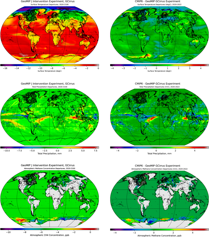
The first vertical panel illustrates weighted mean departures for Tsurf (°C), P (mm day− 1), and subtropospheric multilevel mean of [CH4] (ppb, 300-1,000 hPa) from the fourth GeoMIP experiment (i.e., G7Cirrus). The second vertical panel expands on departure variabilities (i.e., reference period derived from ERA5 reanalysis: 1991–2020) constrained to the observational record (S8). Additional plots for climatologies, departures, statistics, and intercomparison temporal windowing (i.e., G7Cirrus; 2020–2022 [2020–2100]) are provided in S7, S8, and S10, respectively. The plots were generated with Python 3.9.18 and the various modules from the Matplotlib and Cartopy libraries43,44.
Total precipitation events appear localized to the western Arabian Sea equatorial regions and the North Pacific Ocean. However, increasing P trends were observed along the west coast of Jalisco, central Bahia in South America, Uruguay, southern Malawi, and Brisbane. Alternatively, significant dry spells were depicted in the Indian Ocean south of the Bay of Bengal, west of North Sumatra, east of the Philippines (i.e., Guam), and southwestern Colombia. Strong [CH4] anomalies are displayed in the Nord-du-Québec region, along the coast of Terra Nova Bay and the Gerlache Inlet (Amery Ice Shelf), a substantial anomaly near the Ross Ice Shelf in the South Ocean, and finally, localized hot spots in western Kalimantan and North Sumatra. Notable cool spots emerge off the coast of Queen Maud Land (i.e., Utsteinen Nunatak, East Ongul Island).
During ERA5 and G7Cirrus model simulations from 2020 to 2022, Tsurf and P were compared: with climatology removed and spatial averaging applied to compute global mean, we determined that these simulations overestimated the weighted mean of Tsurf (0.02(:pm:)0.32ºC; -2.00-2.12ºC) and underestimated the P (-0.004(:pm:)0.321 mm day-1; -4.27–3.36 mm day-1). Tsurf demonstrated interannual volatility between the simulation and reanalysis data but generalized to a net negative − 0.12(:^circ:)C reduction from 2020 to 2022. Total precipitation revealed similar yet inverted patterns of volatility. Specifically, these patterns illustrated divergent temperatures yielding periods of higher P accuracy, with a generalized diverging net positive trend of 0.05 mm day-1 (i.e., P > ET). Computing the global weighted mean departures for these variables from 2020 to 2022 indicated the model’s tendency to underestimate both Tsurf (-0.61(:pm:)0.02ºC; -4.17-4.72ºC) and P (-0.102(:pm:)0.001 mm day-1; -4.77–5.45 mm day-1) based on temporal bounding conditions in the interest of ERA5 intercomparison efforts. The historical relationships (i.e., 2020–2022) between ERA5-derived and simulated Tsurf and P resulted in global annual weighted mean differences of 1.79(:pm:)0.03ºC and 0.89(:pm:)0.02 mm day-1, respectively. Furthermore, we spatially flattened and temporally differenced the validation data from 1990 to 2022, 1950–2022, and 2020–2022 to generate time series plots and illustrate Tsurf and P variability over 73 years (Fig. 8). These plots demonstrate how model simulations drift from the observational record.
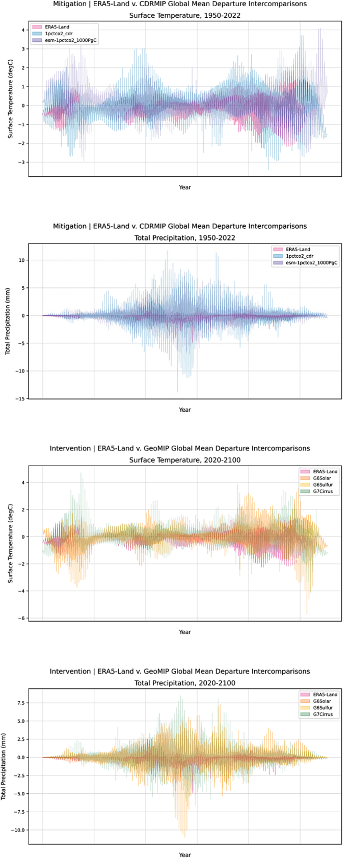
In the top panel, simulation drift is illustrated, thus demonstrating the relationships between Tsurf and P derived from CDRMIP simulations relative to ERA5 reanalysis observations from 2020–2022. Below this panel, the bottom plots illustrate how these covariates (i.e., Tsurf and P) differ not only among various GeoMIP simulations and ERA5 reanalysis data, but also relative to the overlaying plots above, i.e., CDRMIP simulations. The plots were generated with Python 3.9.18 and the various modules from the Matplotlib and Cartopy libraries43,44.
Discussion
This study examined various mitigation and geoengineering experiments to understand these strategies’ potential impacts and identify the most feasible solutions to address global climate change. Some of these experiments included CO2 removal, setting emissions targets, and employing solar dimming, SAI, and cloud seeding technology to reduce solar forcing; these operations and simulation outputs were instantiated and simulated with the UKESM1-0-LL model and compared with ERA5 reanalysis data. In the near term, solar geoengineering strategies could accomplish the brief objective of allowing human management of the solar constant. However, these methods must account for lagged effects from bias and uncertainty originating from Earth system complexities and innumerable multiscale biogeochemical processes. Moreover, potential unintended consequences resulting from each of these geoengineering scenarios are essential to highlight; in particular, Tsurf and P briefly reach – and exceed – stabilization thresholds during the contemporary period in many of these experiments, with rapid warming and increased P, bolstering an enhanced runaway greenhouse effect.
Traditional mitigation approaches primarily focus on reducing GHG emissions to stabilize global temperatures, afforestation, carbon aerosol capture, biochar, and ocean fertilization1,46. Alternatively, market-based instruments include carbon offset incentivization and global carbon accounting approaches (e.g., renewable energy credits). However, current efforts are insufficient to achieve the 1.5 °C climate stabilization target, with global emissions expected to exceed critical thresholds within the next decade. Mitigation strategies often underestimate feedback mechanisms and systemic uncertainties, limiting their effectiveness in stabilizing Earth’s climate systems. Mitigation simulations (e.g., 1pctCO2-cdr) demonstrate reduced Tsurf and altered P patterns in the short term. However, Arctic amplification persists, with pronounced warming in high-latitude regions despite aggressive CO2 reductions. These strategies generally promote gradual stabilization but cannot prevent erratic climate responses entirely.
In contrast, geoengineering involves direct, large-scale manipulation of the Earth’s climate system with SRM and carbon-focused interventions. SRM strategies such as the G6Sulfur sub-experiment demonstrate significant short-term cooling effects while introducing long-term risks, e.g., uneven precipitation patterns facilitate ecosystem disruption, Arctic warming, and equatorial cooling. Other SRM intervention models – including the G7Cirrus sub-experiment – predict marginal Tsurf reductions but highlight P and [CH4] variability, underscoring the complexity of managing interdependent climate systems. Long-term simulations reveal that intervention strategies might exacerbate feedback loops or introduce irreversible climatic shifts when improperly managed. Alternatively, geoengineering intervention via carbon management, including ocean fertilization and enhanced mineral weathering, aims to increase carbon uptake but often encounters substantial ecological uncertainties and unintended consequences, such as hydrological cycle disruption, ocean acidification, biodiversity loss, and ecosystem collapse.
Traditional mitigation strategies offer gradual and predictable outcomes, while geoengineering interventions promise rapid temperature reductions but introduce substantial risks and uncertainties. Mitigation strategies are generally global in scope and balanced in effect, while geoengineering exhibits pronounced regional anomalies (e.g., Arctic warming and equatorial cooling). Mitigation strategies align with natural processes and are more sustainable over the long term. Conversely, geoengineering often requires sustained intervention to maintain results, as abrupt cessation can lead to catastrophic climatic rebound. Geoengineering introduces unknown risks and ethical considerations, such as governance and global equity in impacts, while mitigation emphasizes systemic changes to reduce the root causes of climate change. While mitigation offers long-term sustainability and aligns with global climate stabilization goals, geoengineering provides a rapid but risky pathway to counteract warming trends. Effective climate strategies will likely require an integrated approach, balancing mitigation with carefully regulated geoengineering interventions to address the multifaceted challenges of climate change.
Collectively, intervention and mitigation simulations tended to overestimate the variability and magnitude of Tsurf and P, with substantial regional deviations and scenario-dependent estimation heterogeneity for [CH4]. This highlights the challenges in accurately quantifying and projecting GHG feedback mechanisms. Furthermore, forward projections indicate that both mitigation and intervention scenarios can lead to varied climate responses, emphasizing the complexity and uncertainty in predicting the exact outcomes of different geoengineering strategies. This suggests that model uncertainty may promulgate through the projections but represents a near-to-observational record that is still useful for forecasting. These results demonstrate the efficacy of employing systematic physics-based data-driven methodologies to extend temporal envelopes for exploring multimodal intercomparisons and applying sensitivity analyses to better understand Earth system complexities and highlight potential limitations and unintended consequences of mitigation and intervention strategies. Future efforts will introduce artificial intelligence optimization to enable knowledge discovery and bolster confidence for recommendation and contingency formulation.
Although imperfect compared to observational records, these mitigation and intervention simulation experiments capture large-scale Earth system dynamics well; however, some discrepancies emerge. Utilizing global mean Tsurf and P as points of departure – with the understanding that regional-to-localized dynamics still require more spatially explicit refinement in Earth System Model frameworks – reanalysis and model intercomparisons act as quality assessments and validation baselines to inform calibration updates (i.e., forcing observations, parameterization, drivers) and improve future simulations47. Each model run exhibited unique responses to experiment-specific mitigation (1) or intervention (2) strategies; most importantly, no experimental ‘solution’ produced a stable, steady-state Earth system at any point in time. By introducing geoengineering strategies into the baseline environment, rapid and sustained changes to the Earth system are observed.
1. Mitigation scenarios were simulated to demonstrate the potential of CO2 removal strategies to alter global climatologies in the future substantially; in particular, initialization of the “1pctCO2-cdr“1pctCO2-cdr experiment resulted in global mean climatologies demonstrating consistent increases in Tsurf, P, and [CH4] from 1990 to 2149 (3.89(:pm:)2.62(:^circ:)C, 0.17(:pm:)0.78 mm day-1, 0.01(:pm:)0.27 ppb). In contrast, Tsurf and P were reduced while [CH4] increased from 1990 to 2022 (-0.01(:pm:)0.37ºC, -0.02(:pm:)0.89 mm day-1, 0.02(:pm:)0.25 ppb), suggesting an effective cooling and drying mechanism in the short-term yet vastly underestimates the evolution of Tsurf and P (4.16(:pm:)0.05ºC, 0.98(:pm:)0.01 mm day-1). Critically, this experiment precipitated pronounced Arctic amplification, with Tsurf in excess of 13.08 °C across the tundra and boreal ecotones. In addition, the 1b esm-1pct-brch-1000PgC experiment demonstrated a more balanced climate response with less pronounced increases in global Tsurf, P, and [CH4] from 1950 to 2149 in comparison to 1a, i.e., 0.06(:pm:)0.35ºC, 0.003(:pm:)0.331 mm day-1, 0.001(:pm:)0.169 ppb. However, relative to the entire simulation period, regional variabilities resulted in Tsurf reductions for the 1990–2022 simulation period, with marginal increases in P and [CH4] trajectories (-0.03(:pm:)0.30(:^circ:)C, 0.001(:pm:)0.330 mm day-1, 0.01(:pm:)0.16 ppb). The “esm-1pct-brch-1000PgC” experiment indicates that even under aggressive CO2 removal and carbon management strategies, complex climate feedbacks remain unfettered48.
We extended the distribution curve tails toward a ‘new normal’ by increasing CO2, seemingly magnifying contemporary observed changes of punctuated extreme weather and precipitation49. This variability introduces shifts in regional climates, though it may also be responsible for the increased global warming trend. While the ranges of Tsurf and P in esm-1pct-brch-1000PgC is less than 1pctCO2-cdr, P is increasingly variable in the models, with interannual shifts in P patterns across regions. While the variability of the models at a regional scale may account for some of these outputs, the overall trend towards punctuated P, governed by biogeochemical processes that are not fully captured by the models, is of concern. Moreover, extending the “1pctCO2-cdr” experiment beyond the 1000 PgC benchmark facilitates increasing loss of [CH4] beyond net zero, which may have biogeochemical consequences over time. Regional incongruencies in Tsurf and P are localized to hot and cool dry ecotones exhibiting high net primary productivity and persistent carbon sink-to-source conversion.
2. Various intervention scenarios were explored with numerous geoengineering simulations analyzed, including SRM.
strategies (e.g., solar dimming, stratospheric aerosol injection, cirrus cloud thinning), with many demonstrating the potential to significantly modify Tsurf, P, and [CH4] patterns with varying regional impacts. The G1 experiment (i.e., 4xCO2 and solar dimming) illustrates global radiative balance by reducing solar irradiance to stabilize climatological feedbacks, resulting in significant Tsurf modulations (i.e., slight cooling), extensive variability in P, and increasing [CH4] across the simulated period, i.e., 1850–1949 (-0.01(:pm:)0.47(:^circ:)C, -0.01(:pm:)0.32 mm day-1, 0.003(:pm:)0.180 ppb). However, regional hotspots were distinguishable, with pronounced warming trends and emergent climatic patterns, trends, and anomalies. In the “G6Solar” G6Solar experiment, high-to-medium solar forcing reduction promoted cooling trends, with elevated Tsurf and [CH4] hotspots despite an overall decrease in global mean variability (i.e., departures). Despite reducing Tsurf, P, and [CH4] from 2020 to 2022 (-2.55(:pm:)2.61(:^circ:)C, -0.08(:pm:)0.61 mm day-1, -4.37(:pm:)0.62 ppb) – and cultivating cool, dry spots across the globe in the short-term – Tsurf, P, and [CH4] rebounded and increased over the 2020–2100 simulation period (1.28(:pm:)1.26ºC, 0.05(:pm:)0.35 mm day-1, 1.58(:pm:)1.08 ppb). The “G6Sulfur” experiment (G6Sulfur) aimed to reduce radiative forcing via SAI methods and demonstrated promising results to mitigate warming and cool the planet in the short-term but reduced global P departures (i.e., variability) by doing so. Additionally, the results suggest that this strategy may cause abrupt climatic changes and pose significant long-term stability issues beyond the initial beneficial impacts being achieved, and aerosol effects are diminished. Similarly, the “G7Cirrus” experiment (G7Cirrus) initially facilitated an increase in Tsurf and [CH4], though regional patterns of reduced Tsurf variability were observed. In the long term, the impacts on P variability are significant. Collectively, these results suggest a complex interplay of oscillating dynamics between global, regional, and localized climate regimes and highlight the challenges in forecasting accurate outcomes under mitigation and intervention mechanisms.
“G6Solar” simulation outputs of global weighted mean variabilities indicate synergistic coregulated feedbacks, with persistent trends characterized by abrupt pulses; specifically, [CH4] began and ended the simulation period with net emissions in terms of annual magnitude, but throughout most of the simulation period, [CH4] variability decreased and remained low. In contrast, P variability illustrated anticorrelated behavior, i.e., the simulation period began and terminated with minimal precipitation events and accumulation but rather a steady increase followed by a gradual decrease – in enhanced P variability. Tsurf characteristically stimulates climate feedback patterns governing water vapor distribution and precipitable accumulation. During this validation window, Tsurf and P differencing and dimensionality reduction via spatial flattening demonstrates that over regions with high variability in P, Tsurf departures were marginal and remained stable (i.e., oceans, equatorial tropics); however, less P variability prompted an elevation of Tsurf variability, triggering positive climate feedbacks (i.e., high latitudes). These trends remained periodic with gradual increases in Tsurf and P – in concert with net release yield from [CH4] – through the end of the century, followed by a slight stabilization period.
Marked reductions in global mean departures from “G6Solar” simulations suggest this strategy will cool the planet while synergistically amplifying the positive coupling feedbacks between Tsurf and P, fostering cool, drier conditions. Examining global climatologies and mean departures for each of the covariates indicate similar characteristics to prescribed solar geoengineering scenarios, with marked increases in global weighted mean variability for P variability across the entirety of eastern Brazil – from Bahia to São Paulo – as well as Tsurf and [CH4] anomalies near the Ross and Amery Ice Shelf. Results from these simulations are shockingly similar to those derived from the previous experiment; however, when constraining and comparing these dynamics with a three-year period and examining global response, subtle nuances between experimental methods are blanketed by statistical liberties. These nuances are not readily discernible in the second panels illustrated in Figs. 5 and 6, both yielding nearly identical visual outputs; however, it is important to note that this three-year window is a sensitivity method for validation purposes and successfully demonstrates similar spatiotemporal dynamics with those observed and re-analyzed datasets. Moreover, the global mean variability between the two experiments from 2020 to 2100 results in strikingly different outcomes, thus illustrating how climatologies change, anomalies evolve, and land-ocean-atmospheric interactions over space and time foster global climate change. Tsurf variability in “G6Solar” is likely coupled with unique surface flux exchanges and biogeophysical dynamics. However, it is more likely associated with the erratic variability of P. SAI, which has the potential to mitigate solar irradiance within Earth’s atmosphere for a finite amount of time. The model results respond accordingly, with steady, linear, and increasing Tsurf and P for the first 30 years after initialization, followed by an abrupt increase in global mean Tsurf. These dynamics may be caused by feedback interactions with the Earth systems or due to progressive atmospheric sulfate loss. Still, the stabilization of the system with abating temperatures, even in the absence of fossil fuel reductions, is concerning, especially when abrupt increases occur. This strategy exhibits less.
interannual variability and challenges long-term climate stability.
Relative to baseline simulations, SAI methods facilitate similar trends to these patterns. However, the magnitude of P’s global weighted mean variability is significantly higher as a consequence of G6Solar, while Tsurf exhibits lower variability. In addition, “G1” and “G6Solar” produced anticorrelated covariate trends, with G1 showing higher variability of Tsurf, P, and [CH4]. This is due to solar irradiance reduction techniques. The G1 experiment created a broad reduction in variable magnitude but demonstrated how reduced variability does not necessarily foster and maintain Earth system stability. This experiment yields a poorly distributed and relatively static lower atmosphere with less fluidity and more turbidity (i.e., amplified hot and cool dry regions, Antarctic methane pooling). These two approaches address and resolve uncertainty challenges by altering light or matter. Another case of an anticorrelated covariate trend is G6Sulfur and 1pctCO2-cdr: “G6Sulfur” induces a reduction in Tsurf and [CH4] variability while increasing P variability on a global scale. In contrast, 1pctCO2-cdr increases Tsurf variability coupled with a less variable global weighted mean in P. The variability of the global weighted mean of [CH4] was significant during G6Sulfur, representing nearly four orders of variable magnitude relative to [CH4] output variability from 1pctCO2-cdr. The dissimilar system responses reiterate that small perturbations can have significant effects when magnified across space and time. During the G7Cirrus experiment, the global mean Tsurf is reduced considerably. The elevation in P may be marginal, but the variance has a long tail toward positive, which could result in considerable precipitation increases over time. The mean cooling response from this experiment requires more time than the others, reaching the maximum radiative and cooling benefit over 160 years.
Based on the observed record, model simulations, sub-experiment intercomparisons, and statistical analyses, potential mechanisms and drivers of change are explored and elucidated within spatiotemporal patterns, relationships, and trends. First, warming departures in Greenland and northern Siberia facilitate land-atmosphere interactions through arctic amplification due to reductions in snow and ground ice, subsequent albedo reduction, and coincident amplification of solar energy absorption and land Tsurf. Hot spot anomalies – in particular, Tsurf departure anomalies – may be a byproduct of equatorial and polar temperature gradient reductions contributing to a weakening of the polar jet stream resulting from the reduction of the temperature gradient. With amplified surface warming and accelerating permafrost degradation, a higher rate and magnitude of [CH4] release from thawing permafrost contributes directly to localized weather patterns. [CH4] departures are located in model diagnostics to isolate and, more explicitly, identify drivers of regional warming. We quantify albedo changes and feedback amplification using remote sensing and process-based models to disentangle driving mechanisms and reconcile algorithm, data, and knowledge gaps.
Furthermore, SRM deployment may alter the cloud cover and radiative balance in high-latitude ecotones due to immediate cooling effects. Alternatively, warming departures in the Horn of Africa may facilitate ocean-atmosphere interactions in the form of alterations to sea surface temperatures (SSTs) in the Indian Ocean, disrupt monsoon systems, and catalyze warmer weather with sporadic precipitation activity. Demonstrating the validity of this conjecture would require coupled oceanic and atmospheric models to assess an SST-driven impact on regional climatological variability. Additionally, persistent drought events were observed and simulated in this region; these disturbances and conditions elevate surface albedo via soil desiccation, reducing latent heat flux and promulgating heat intensification. Moreover, model parameterization, including soil moisture and vegetation feedbacks, would enhance the model architecture, increase the precision of the simulation outputs, and reduce uncertainties and confidence intervals that directly validate and support drivers of change.
Cooling mechanisms and drivers of change are further examined; in particular, central Africa and eastern Brazil experienced significant regional cooling effects. Drivers contributing to regional cooling departures in central Africa may result from vegetation feedbacks and changes to the hydrological regime; more specifically, afforestation catalyzes an increase in evapotranspiration and latent heat flux, effectively cooling Tsurf. Though enhanced forest cover may be a minute contributor, this hypothesis may be validated by integrating dynamic vegetation models into the coupled terrestrial and atmospheric circulation models to simulate land-atmosphere interactions while conducting cooling effect assessments effectively. In contrast, moisture transport variability may result from altered trade wind patterns, thereby increasing P and promulgating evaporative cooling; similarly, this hypothesis may be tested with remote sensing platforms that observe water vapor flux and cloud cover variability. Alternatively, the historical rate and magnitude of deforestation in eastern Brazil across the Amazon basin may help contribute to localized cooling patterns via reduced transpiration and latent heat flux (i.e., land-use land-cover change scenarios may be used to emulate and assess the interplay among the spatiotemporal dynamics of deforestation and Tsurf trends across this region). In addition, cooling effects in eastern Brazil may be a result of the circulation pattern of the Atlantic Ocean; more specifically, disruptions to the Atlantic Meridional Overturning Circulation (AMOC) would drastically affect heat transport to the tropics. Simulating this scenario with AMOC variations in response to various geoengineering intervention strategies would validate and effectively constrain potential states of the regional climate.
Discrepancies between the observational record, model simulations, and statistical products are present, most notably acknowledged previously as over- and under-estimations of simulated outputs and observed data. In particular, P was overestimated in southern Alaska, while P was underestimated in east Africa. First, we expound on potential climatological, geophysical, and biogeochemical contributors to these errors; then, we expand these inquiries to technological limitations. The error or overestimation of P in southern Alaska may be a result of marine-dominated regimes; in particular, warm SSTs in the North Pacific may expedite a significant amount of moisture and heat transport to southern Alaska (i.e., atmospheric river), prompting the development of thunderstorms and excessive precipitation. Alternatively, if warm SST in the North Pacific does not fuel the system, model simulations and architectures may not accurately reflect orographic effects or convective processes. Instead, much of the overestimation error and biases likely originate from inadequately accounting for and capturing the dynamics of cloud microphysics and convective processes. To remedy this, adapting high-resolution cloud-resolving models into the coupled oceanic and atmospheric circulation models to better resolve and improve the representation of orographic P.
The underestimation of P in East Africa may be a byproduct of generalized downsampling; however, the inability to capture and simulate localized convection and mesoscale phenomena at coarse resolution may contribute iteratively to the resulting error and underlying biases. Furthermore, this underestimation of P may result from poor representation of monsoon dynamics in simplified parameterizations of moisture convergence and seasonal wind shifts. Integrating observational datasets for model calibration purposes would reduce errors and biases significantly. Broader structural constraints and model limitations may directly contribute to these P errors via parameterization errors and feedback mechanisms; however, spatial resolution was not a contributing factor in this context (i.e., preprocessing methodology guided by ERA5 resolution). By refining parameterizations, updating simplified assumptions generalizing cloud formation, radiation, and convection – and interjecting complexity with satellite cloud retrievals and ground-based radar data – regional climate simulations will contain fewer biases and output more precise data products. Amending the represented feedback mechanisms in coupled Earth system model frameworks is crucial as well to enhance the predictive accuracy of the simulations (e.g., vegetation-climate, ocean-atmosphere).
Climate change remains a critical issue, and the likelihood of geoengineering intervention in the future is likely. Geoengineering represents an unprecedented scale of planetary intervention, carrying profound implications and the risk of significant consequences. It is a field marked by considerable uncertainties that can only be addressed through systematic and coordinated research efforts. In addition, while CDR strategies are integral to many climate change mitigation scenarios, their development has yet to achieve the necessary deployment scale required for climate change mitigation, and their impacts on the Earth system still need to be better understood. Through detailed simulation analyses, this research study – presuming other approaches to this challenge are generalized and not comprehensive – identified substantial variability in global, regional, and localized climate patterns from ERA5 reanalysis observations over 73 years (i.e., 1950–2022) as well as six mitigation and intervention simulations from CMIP6 experiments (i.e., CDRMIP, GeoMIP) from 1850 to 2149, reflecting complex hydrological responses to changing atmospheric conditions. While the experiments provide valuable insights into potential strategies for managing climate change, they also reveal the complexities and uncertainties involved, necessitating further research and cautious approaches to large-scale implementation of geoengineering solutions.
Geoengineering strategies are intrinsically characterized by significant uncertainties, those which critically govern and influence decision-making processes by shaping the evaluation of risks, trade-offs, and potential unintended consequences. Empirical, temporal, technological, ethical, and socioeconomic uncertainties permeate from various stages of geoengineering deployment, from regional climate responses to governance and moral challenges. Ethical and governance issues arise from these uncertainties, significantly influencing international cooperation and policy frameworks. Intervention often produces unequal regional impacts, e.g., the G7Cirrus sub-experiment, which illustrates increased P variability in equatorial regions but induces drying patterns in parts of southeast Asia and Brazil. Quantitative evaluations, including the (:pm:)1Wm-2 radiative forcing reduction in cloud-seeding sub-experiments, inform the design of equitable governance frameworks to address these disparities. Additionally, uncoordinated regional deployment of cloud-seeding efforts highlights the risks and pressing need for global regulatory mechanisms. While cloud-seeding experiments suggest radiative forcing reductions of 50–85%, geographic variability in outcomes necessitates comprehensive oversight. Uncertainties from geoengineering outcomes arise due to an incomplete understanding of Earth system processes, model limitations, and potential unintended consequences. Model simulations such as the G6Sulfur experiment illustrate erratic regional climate responses, with P departures ranging from − 2.22 mm day-1 to 3.13 mm day-1 globally. Regions such as eastern Brazil experience extreme drying, while high-latitude areas exhibit increased P variability, complicating regional projections. Similarly, [CH4] dynamics and sensitivity to atmospheric chemistry variability add to the complexity; G6Sulfur simulations indicate global mean [CH4] variability between − 4.43 ppb and 6.38 ppb, raising concerns about activation and amplification of nonlinear feedback loops, particularly in methane-sensitive regions. These regional disparities compel policymakers to weigh localized risk against global cooling benefits, underscoring the cautious approach policymakers adopt. This complicates large-scale deployment consensus and includes the implementation of well-informed decisions and actionable task delegation that minimizes risk and maximizes utility and efficiency, ultimately seeking to diminish feedback-driven warming while prioritizing adaptation and mitigation approaches.
These results and uncertainties quantified from erratic regional climate response patterns and [CH4] dynamics collectively impact and govern decision-making processes. Moreover, these wide-ranging outcomes make it challenging to predict how regions will respond and adapt to driving factors and covariate departures, which inherently lead policymakers to approach geoengineering decision-making with caution. Another challenge regarding geoengineering deployment is the uncertainty representing each strategy’s efficacy and uneven regional impacts, challenges that often result in hesitancy regarding policy timing, risk assessment, and deployment. Unpredictability and unwavering uncertainties characterize intervention strategies motivate policymakers to favor established alternative mitigation strategies until these uncertainties and confidence intervals are better constrained. Moreover, the risk of catastrophic rebound from intervention highlights the temporal dependencies illustrated by geoengineering approaches; more concretely, if intervention ceases abruptly, global mean Tsurf may rise sharply and catalyze climatic shocks​. Consequently, policymakers are inclined to mandate parallelized mitigation approaches to reduce the reliance on interventions and dependencies while suppressing potential climatic shocks with sustained sequestration efforts.
The potential benefits of geoengineering must be weighed against its associated risks and uncertainties through cost-benefit analyses, i.e., SAI strategies show promise for global cooling but risk destabilizing precipitation patterns and disproportionately affecting agriculture-dependent economies. Cooling effects exhibit significant uncertainty; e.g., the G1 experiment predicts Tsurf reductions of -6.87 °C to 4.38 °C with uneven regional distributions​. G6Sulfur results demonstrate a global P increase of 0.03 mm day-1, contrasted with a -1.20 mm day-1 reduction in East Africa, posing significant regional drought risks​. Temporal dynamics further complicate these analyses, i.e., solar dimming approaches, i.e., the G6Solar sub-experiment, provide cooling effects lasting 80–120 years. However, this comes at the cost of long-term dependencies on continuous intervention, which policymakers find unsustainable​ in general. Risk-reward balancing is another mechanism to guide climate policy; in particular, the 1pctCO2-cdr sub-experiment explores arctic amplification and reveals Arctic warming up to 13.08 °C, far exceeding global mean changes, thus accelerating permafrost thaw and methane release​. This unabated warming in the Arctic and the activation of multiple feedback loops emphasize the need for Arctic-specific geoengineering trials, such as localized aerosol injections, to mitigate these nonlinear runaway effects. In addition, intervention escalation risks are identified, and an intervention escalation risk framework is adopted, e.g., the abrupt cessation of SAI may result in warming rates of up to 1.5 °C per decade, with catastrophic ecological consequences​. Dual strategies combining emissions reduction and geoengineering could mitigate reliance on high-risk interventions.
Uncertainty requires iterative enhancement and application of sensitivity analyses and model architecture refinements to update, bolster, and improve model performance while reducing uncertainty and increasing confidence in geoengineering proposals (e.g., Tsurf variability of ± 2.55 °C in G6Solar simulations underscores the need for region-specific models​). Policymakers increasingly rely on such analyses to guide incremental deployment or pilot testing. Phased approaches to geoengineering allow policymakers to target regions where benefits outweigh risks while implementing pilot testing, small-scale trials, and conditional deployment for risk mitigation. Policies may also link deployment to predefined thresholds, such as global temperatures exceeding 2.0 °C. Quantitative examples from model simulations highlight the guiding policies that prioritize mitigation and adaptation, invest in model refinement, integrated assessment model development, and state-of-the-art research, bolster multilateral governance frameworks, manage shared risks (i.e., delicate trade-offs between potential benefits and risks), and ensure equitable outcomes. By addressing these uncertainties, policymakers are better positioned to address scientific, ethical, and geopolitical challenges. Examples of quantitative insight derived from this study are iterated below to demonstrate policy responses to climatological trends: P variability necessitates regional pilot studies with controlled P monitoring, i.e., G6Sulfur simulations indicate global P anomalies of ± 2.5 mm day-1 with regional drought risk probabilities; delay SAI deployment until [CH4] dynamics are more universally and comprehensively understood, i.e., [CH4] magnitude ~ 6.38 ppb exacerbates warming in defined regions; adaptation and mitigation mandate serve as a backup to avoid intervention overreliance, with abrupt SAI cessation leading to a 1.5 °C decade-1 warming rate.
The contributions and sources of error resulting in simulated over- and underestimations may originate from computational methods, statistical limitations (e.g., climatological mean, temporal windowing), lack of variant ensemble diversity, spin-up perturbations, generalized parameterization, and new data assimilation techniques that impose new conditions on the system with restrictions and potential information loss from scaling efforts. To reduce possible errors and uncertainties originating from coarsely resolved scaling practices, ongoing efforts will prioritize stability and consistency by incorporating a multi-model multi-variant ensemble (i.e., UKESM1-0-LL, CanESM5, CNRM-ESM2-1, MIROC-ES2L, MPI-ESM1-2-LR) while introducing cutting-edge methodologies to reduce uncertainties and bolster validation efforts prior to 1950 – including artificial intelligence (AI), machine learning (ML), and AI optimization (AIO) frameworks – to better quantify and understand dynamics, patterns, and trends that emerge over time. These methodologies will enable knowledge discovery and confidence for recommendation systems and contingency formulation while offering the potential to optimize geoengineering designs by simulating nonlinear dynamics, analyzing large datasets with various data harmonization and assimilation frameworks, and minimizing risks with a multimodal neural network architecture.
An AIO implementation plan is defined by algorithm selection, data integration, and validation criteria to enhance the utility and rigor of these tools and methodologies. Suitable algorithms for geoengineering AIO tasks include reinforcement learning for SAI optimization, convolutional long short-term memory recurrent neural network (ConvLSTM) for spatiotemporal feedback prediction, variational autoencoders for reducing the dimensionality of massive climate datasets and process-based modeling outputs, and Bayesian optimization for uncertainty quantification during model predictions. For demonstration purposes, the data preprocessing workflow consists of training and testing the ConvLSTM network with historical SST, P, and atmospheric pressure data assimilated from MODIS observations, high-resolution ERA5 reanalysis data, and CMIP6 multi-model ensemble outputs. After training, validation protocol (e.g., cross-validation with independent climate data records), cost functions (RMSE, MAE), and skill scores are implemented to correct simulation biases or assess the fidelity, resilience, and reliability of regional climate feedback predictions generated from upsampled geoengineering intervention scenarios. Baseline quantities and these validation metrics not only assist with defining benchmarks for model agreement and bias detection, i.e., simulated v. observed intercomparisons but also improve existing and future climate feedback representations in model architecture while enhancing G6Solar and G6Sulfur simulations.
AI methods serve a critical role in optimizing geoengineering strategies since they can rapidly analyze massive numbers of scenarios to help identify the strategies that minimize risks and unintended consequences. However, AI introduces its own uncertainties, such as biases in feature selection and interpretability challenges​, necessitating a balanced approach to integrating AI into decision-making processes. Additionally, the integration of AI into geoengineering playbooks presents inherent risks that are not yet fully understood35. These unknown risks and impacts may originate from a flawed optimization question, deploying imperfect algorithms in haste, or applying imperfect toolkits to an incomplete feature space with a flawed understanding of the Earth system. In light of persistent knowledge gaps, a dearth of observations, and industry standardized uncertainty quantification methodologies falling short, AIO strategies help address these areas of improvement while enhancing model performance. AI provides a powerful optimization tool, and the decision to implement a particular AIO algorithm is intrinsically an optimization question void of equifinality that concerns quality, performance, cost, and tractability50. We advocate for continued research into the efficacy, limitations, and implications of various climate intervention methods, emphasizing the need for a more comprehensive understanding of climate dynamics and calling for more refined models and international collaboration to mitigate the exacerbation of existing climate risks and strategically manage the potential irreversible impacts of global climate change.
Methods
We utilized ERA5 reanalysis data as well as mitigation (i.e., CDRMIP) and intervention (i.e., GeoMIP) simulations first to examine baseline conditions to gain a retrospective understanding of climate warming and then prognosticating climate response patterns under a variety of mitigation and climate engineering scenarios. We compared observation-based ERA5 reanalysis data with simulation outputs from the CDRMIP and GeoMIP experiments. The temporal bounds of the simulation experiments were constrained to the observational period (i.e., 1950–2022) for Tsurf and P intercomparisons (i.e., 1pctCO2-cdr), 1950–2022 (i.e., esm-1pct-brch-1000PgC), and 2020–2022 (i.e., G6Solar; G6Sulfur; G7Cirrus).
The UKESM1-0-LL model (i.e., r1i1p1f2 ensemble member) was selected for this study because it is one of only six projects involved with simulating both mitigation and climate engineering scenarios (i.e., CDRMIP, GeoMIP) while offering a breadth of ensemble variants and surface variables at various temporal resolutions on a Native N96 grid. For sensitivity analyses, P simulations derived from these simulations were converted to P (i.e., kg m−2 s−1 to mm day−1) based on temporal windowing and the global surface basin. In addition, the subtropospheric multilevel mean of [CH4] was converted to parts per billion (i.e., mol mol−1 to ppb).
ERA5 Reanalysis
ERA5 Reanalysis observations (e.g., Tsurf, P) were regridded from (721, 1440) at 0.25° resolution with 3.88B samples to (143, 191) at 2.348° resolution with 16.03M observations (i.e., 27320 global observations per annum). The standard reference period as defined by the WMO identifies climate normal (i.e., 1991–2020); however, ERA5 Reanalysis data utilizes 1981–2010 as a base period; therefore, we selected this time period, i.e., 1981–2010. ERA5 monthly averaged high-dimensional reanalysis datasets were extracted from the European Centre for Medium-Range Weather Forecasts Climate Data Store portal generated by Copernicus Climate Change Service. The CDS API tool was utilized to efficiently query the database with appropriate parameters in place, i.e., global coverage over a 73-year period. Following regridding and scaling, these datasets were loaded, concatenated, and restructured into a dataframe.
CMIP6 Simulations
In addition, 699.72 M modeling outputs including abiotic measurements, e.g., Tsurf, P, and [CH4] derived from CMIP6 projects including the Geoengineering Model Intercomparison Project (i.e., GeoMIP) and the Carbon Dioxide Removal Model Intercomparison Project (i.e., CDRMIP) experiments (i.e., concluding NaN dropping via bilinear interpolation, backfilling, and forward-filling, 341.40 M and 358.32 M, respectively). Subsets of these experiments were searched and downloaded from the LLNL metagrid node with the ESGF PyClient API.
Many geoengineering and CO2 removal intercomparison scenarios adopt sophisticated architectures and assessment protocols (e.g., CDRMIP, GeoMIP). However, mitigation efforts are limited in scope and often formulate uninformed strategies based on single high-emissions pathways inconsistent with near-term projections. The CDRMIP project aims to consolidate Earth system models within a unified framework to evaluate the feasibility, effects, and challenges associated with CDR technologies. The GeoMIP project aims to meet this research need by standardizing sub-experiments across participating climate models. This initiative will enable the identification of both commonalities and discrepancies of climate response to mitigation and intervention in model predictions, thereby contributing vital insights into potential outcomes of significant global efforts.
We examined mitigation and intervention strategies employed by assessment protocols and SSP scenarios to identify global historical and future relationships and climate change indicators from 1850–2149 (e.g., Tsurf, P, and [CH4]). Due to escalating extreme events and more support growing for weather modification tactics, it was necessary not only to examine anomalies, trends, and bounds of the datasets but to also constrain the temporal look-forward period to 2050 in the interest of expedient mitigation and policy implementation. We examined these experimental runs from 1850 to 2149, with careful scrutiny given to periods of data misalignment and natural disturbance events (e.g., Pinatubo), and further examination during the years 2020 and 2050, notating critical information that may prove useful in terms of deployment and policymaking.
A more comprehensive list of results distributed by experiment, period, covariate, and uncertainty is provided in the Data Availability Statement. GeoMIP simulations were analyzed to understand the historical and future implications of current strategies and the potential consequences of implementing geoengineering practices. Baselines were established to provide historical lenses (i.e., G1) and real-world atmospheric forcing (i.e., ERA5) to determine the feasibility of contemporary geoengineering proposals and the associated impacts on the Earth system over time. Concluding initial baseline runs, we extended the temporal retrospection period by 100 years with historical simulations (i.e., 1850–1949, G1) and the prognostication period by 77–128 years with forward projections of intervention (i.e., 2023–2100, G6Solar, G6Sulfur, G7Cirrus) and mitigation experiments (i.e., 2023–2149, 1pctCO2-cdr, esm-1pct-brch-1000PgC).
Data preprocessing
These data products were loaded, appended, scaled, and reframed in each experiment-specific sequencing of the dataframe (i.e., CDRMIP: (199065600, 5)1PCT), GeoMIP: (80621568, 5)G1, (159252480, 5)GSSC) prior to assimilating with observation-derived ERA5 data with a bilinear periodic regridding algorithm (i.e., xESMF Regridder) to improve performance, compatibility, and interpretability. CMIP6 experiments yield daily outputs, prompting monthly mean resampling across these simulation datasets to align with ERA5 reanalysis monthly observations. These dataframes were concatenated along the temporal dimension, resulting in a (23951989, 93) dataframe with 93 variables obtained from ERA5 reanalysis data across 1950–2022 (i.e., Tsurf, P), CDRMIP 1pctCO2-cdr and esm-1pct-brch-1000PgC experiments from 1950–2022 and 1990–2022 respectively (i.e., Tsurf, P, [CH4]), GeoMIP G1 spin-up simulations from 1850–1949 (i.e., Tsurf, P, [CH4]), and GeoMIP G6 and G7 geoengineering experiments from 1850–2100.
-
ERA5 global monthly averaged observations (e.g., Tsurf, P): 24.25 M regridded data points from 1950–2022.
-
CRU TS4.08 (Climatic Research Unit Time-Series version 4.08) high-resolution global monthly observations (e.g., tmp, pre): 118.12 M gridded data points from 1950–2022.
-
1pctCO2-cdr: In the wake of 4×CO2 preindustrial baseline, one percent CO2 reduction per year is prescribed until preindustrial control is reached and maintained (1990–2149)
-
esm-1pct-brch-1000PgC: After 1000 Pg cumulative emissions threshold is achieved, zero emissions are simulated after 1pctCO2-cdr run (1950–2149)
-
G1: 4×CO2 mitigation via solar radiation management (1850–1949)
-
G6Solar: High forcing scenario reduction to medium forcing via solar radiation management, i.e., solar irradiance reduction (2020–2100)
-
G6Sulfur: High-to-medium forcing scenario reduction; sulfate aerosol injection, SAI (2020–2100)
-
G7Cirrus: High forcing scenario baseline mitigation via increases in rate and magnitude of cirrus ice crystallization, i.e., cloud seeding (2020–2100)
Intrinsic biases within the ERA5 reanalysis dataset were addressed with temporal resampling, weighted climatological mean deviations from the baseline, climatological departures and anomalies, and bias-corrected uncertainty quantification. Global mean products, regional variability patterns, data-driven biases, and coincident trending impacts were inferred from CRU TS4.08, ERA5, and CMIP6 intercomparisons (e.g., elevated Tsurf in Greenland v. cooling anomalies in central Africa). To address the potential intrinsic, aleatoric, and empirical biases affecting the baseline Tsurf and P in the ERA5 reanalysis dataset, we compared resampled ERA5 reanalysis data, including 2 m Tsurf and P against globally gridded in situ observations extracted from the CEDA archive (CRU TS4.08). Biases were quantified utilizing cost functions – more specifically, mean square error (MAE), root mean square error (RMSE), and other statistical testing (MAPE, R) – while discrepancies and uncertainties were corrected by aligning ERA5 with observed distributions via sorting, ranking, smooth interpolation, and quantile mapping (i.e., 1950–2022). These corrections to ERA5 data were validated through cross-validation methods resulting in an improved agreement between Tsurf and P variability from ERA5 reanalysis data and CRU TS4.08 observations (i.e., for Tsurf, MAE was reduced by 13.55% [3.03°C to 2.62°C] and RMSE was reduced by 13.78% [3.86°C to 3.33°C] while validation metrics for P vastly improved: MAE was reduced by 98.07% [60.68 mm day−1 to 1.17 mm day−1] and RMSE was reduced by 97.76% [103.73 mm day−1 to 2.327 mm day−1]).
Concluding bias quantification, correction, and validation, ERA5 was used as the observational baseline to compare mitigation and intervention sub-experiments To ensure temporal consistency, monthly means of Tsurf and P derived from ERA5 reanalysis data were resampled and regridded to align with temporal windows characterizing the CMIP6 sub-experiments. Each of the six sub-experiments contains set-specific biases and errors wherein uncertainties in the CMIP6 multi-model ensemble were quantified by utilizing validated ERA5 reanalysis bias-corrected Tsurf and P data, and the combined six sub-experiment aggregations of regridded interquartile-ranged bias-corrected validated weighted mean of Tsurf and P. From 1950–2022, after reconciling mismatched lengths due to missing values, partial temporal overlaps, and interpolation artifacts, the multi-model ensemble uncertainties computed from observation-model metrics (i.e., Root Mean Square Error, RMSE; Mean Absolute Error, MAE; Nash-Sutcliffe Efficiency, NSE; Pearson’s Correlation, r) resulted in 276.08 K, 276.03 K, −233.75, and 96.80 respectively for Tsurf and 2.65 mm month−1, 1.40 mm month−1, 0.05, and 59.57 respectively for P.
Ongoing work examines these covariates with retrospective and prognostic purviews, i.e., G6 and G7 experiments (2023–2149) and OSCAR v3.3 modeling output (2023–2100) will serve as proxies for testing the prediction abilities of the model (i.e., seasonal, annual, decadal, semicentennial) while accounting for model drift anomalies that exhibits the potential to propagate in space and time. In addition, employing testing data helps identify key temporal relationships that may provide a more comprehensive understanding of local-to-regional effects of disaggregation and down-sampling methods to further disentangle anomaly detection (i.e., localizing trend and feedback dynamics that require data-informed scenario-based decision-making).
Datasets
Repositories, data archives, simulation results, and synthesis work are publicly available (GitHub, JPL DOI). Many of the state, diagnostic, and prognostic variables are inferred and/or derived from global annual mean mixing ratios, harmonized emissions, global annual mean radiative forcing, SSP-based simulations and scenario projections (i.e., SSPs), and subsequent geoengineering experiments (e.g., GeoMIP, CDRMIP). The corresponding models, variables, and frequencies are enumerated in the Supplementary Information.
Observations and reanalysis datasets
CRU TS4.08: Independent observations derived from CRU TS4.08 were used for validation purposes: University of East Anglia Climatic Research Unit; Harris, I.C.; Jones, P.D.; Osborn, T. (2024): CRU TS4.08: Climatic Research Unit (CRU) Time-Series (TS) version 4.08 of high-resolution gridded data of month-by-month variation in climate (Jan. 1901- Dec. 2023). NERC EDS Centre for Environmental Data Analysis, 1 December 2024 https://catalogue.ceda.ac.uk/uuid/715abce1604a42f396f81db83aeb2a4b/
-
CRU TS4.08 temperature: https://data.ceda.ac.uk/badc/cru/data/cru_ts/cru_ts_4.08/data/tmp
-
CRU TS4.08 precipitation: https://data.ceda.ac.uk/badc/cru/data/cru_ts/cru_ts_4.08/data/pre
ERA5: Hersbach, H., Bell, B., Berrisford, P., et al. The ERA5 global reanalysis. Q J R Meteorol Soc. 2020; 146: 1999–2049. https://doi.org/10.1002/qj.3803
-
Hersbach, H., Bell, B., Berrisford, P., Biavati, G., Horányi, A., Muñoz Sabater, J., Nicolas, J., Peubey, C., Radu, R., Rozum, I., Schepers, D., Simmons, A., Soci, C., Dee, D., Thépaut, J-N. (2023): ERA5 monthly averaged data on single levels from 1940 to present. Copernicus Climate Change Service (C3S) Climate Data Store (CDS), DOI: https://doi.org/10.24381/cds.f17050d7 (Accessed on 24-Mar-2024).
Activity nodes
CMIP5 Scenarios (RCPs): https://www.pik-potsdam.de/~mmalte/rcps
CMIP6 Scenarios (SSPs): ScenarioMIP: https://aims2.llnl.gov/search
CMIP6 Experiments (MIPs): CDRMIP, GeoMIP: https://aims2.llnl.gov/search
Models
ScenarioMIP (59 Models): ACCESS-CM2, ACCESS-ESM1-5, AWI-CM-1-1-MR, BCC-CSM2-MR, CAMS-CSM1-0, CAS-ESM2-0, CESM2, CESM2-FV2, CESM2-WACCM, CIESM, CMCC-CM2-SR5, CMCC-ESM2, CNRM-CM6-1, CNRM-CM6-1-HR, CNRM-ESM2-1, CanESM5, CanESM5-1, CanESM5-CanOE, E3SM-1-0, E3SM-1-1,E3SM-1-1-ECA, E3SM-2-0, EC-Earth3, EC-Earth3-AerChem, EC-Earth3-CC, EC-Earth3-Veg, EC-Earth3-Veg-LR, FGOALS-f3-L, FGOALS-g3, FIO-ESM-2-0, GFDL-CM4, GFDL-ESM4, GISS-E2-1-G, GISS-E2-1-G-CC, GISS-E2-1-H, GISS-E2-2-G, HadGEM3-GC31-LL, HadGEM3-GC31-MM, IITM-ESM, INM-CM4-8, INM-CM5-0, IPSL-CM5A2-INCA, IPSL-CM6A-LR, KACE-1-0-G, KIOST-ESM, MCM-UA-1-0, MIROC-ES2H, MIROC-ES2L, MIROC6, MPI-ESM-1-2-HAM, MPI-ESM1-2-HR, MPI-ESM1-2-LR, MRI-ESM2-0, NESM3, NorESM2-LM, NorESM2-MM, TaiESM1, UKESM1-0-LL, UKESM1-1-LL, https://pcmdi.llnl.gov/CMIP6/ArchiveStatistics/esgf_data_holdings/ScenarioMIP/
CDRMIP (12 Models): ACCESS-ESM1-5, CanESM5, CanESM5-CanOE, CAS-ESM2-0, CESM2, CNRM-ESM2-1, GFDL-ESM4, GISS-E2-1-G-CC, MIROC-ES2L, MPI-ESM1-2-LR, NorESM2-LM, and UKESM1-0-LL, https://pcmdi.llnl.gov/CMIP6/ArchiveStatistics/esgf_data_holdings/CDRMIP/
GeoMIP (8 Models): CanESM5, CESM2-WACCM, CNRM-ESM2-1, IPSL-CM6A-LR, MIROC-ES2H, MPI-ESM1-2-HR, MPI-ESM1-2-LR, and UKESM1-0-LL, https://pcmdi.llnl.gov/CMIP6/ArchiveStatistics/esgf_data_holdings/GeoMIP/
CDRMIP Experiments | UKESM1-0-LL r1i1p1f2 member
1pctCO2-cdr: 1 percent per year decrease in CO2 from 4×CO2https://doi.org/10.22033/ESGF/CMIP6.12183
CMIP6.CDRMIP.MOHC.UKESM1-0-LL.1pctCO2-cdr.r1i1p1f2.Amon.ts.gn.v20200425|esgf.ceda.ac.ukpr
CMIP6.CDRMIP.MOHC.UKESM1-0-LL.1pctCO2-cdr.r1i1p1f2.Amon.pr.gn.v20200425|esgf.ceda.ac.uk[CH4]
CMIP6.CDRMIP.MOHC.UKESM1-0-LL.1pctCO2-cdr.r1i1p1f2.Amon.ch4.gn.v20200425|esgf.ceda.ac.uk
esm-1pct-brch-1000PgC: Zero emissions simulation branched from 1 percent run after 1000 PgC cumulative emission https://doi.org/10.22033/ESGF/CMIP6.10785
CMIP6.C4MIP.MOHC.UKESM1-0-LL.esm-1pct-brch-1000PgC.r1i1p1f2.Amon.ts.gn.v20200210|esgf.ceda.ac.ukpr
CMIP6.C4MIP.MOHC.UKESM1-0-LL.esm-1pct-brch-1000PgC.r1i1p1f2.Amon.pr.gn.v20200210|esgf.ceda.ac.uk[CH4]
CMIP6.C4MIP.MOHC.UKESM1-0-LL.esm-1pct-brch-1000PgC.r1i1p1f2.Amon.ch4.gn.v20200210|esgf.ceda.ac.uk
GeoMIP Experiments | UKESM1-0-LL r1i1p1f2 ensemble member:
G1
Abrupt quadrupling of CO2 plus a reduction in total solar irradiancehttps://doi.org/10.22033/ESGF/CMIP6.5812 ts
CMIP6.GeoMIP.MOHC.UKESM1-0-LL.G1.r1i1p1f2.Amon.ts.gn.v20190916|esgf.ceda.ac.uk pr
CMIP6.GeoMIP.MOHC.UKESM1-0-LL.G1.r1i1p1f2.Amon.pr.gn.v20190916|esgf.ceda.ac.uk[CH4]
CMIP6.GeoMIP.MOHC.UKESM1-0-LL.G1.r1i1p1f2.Amon.ch4.gn.v20190916|esgf.ceda.ac.uk
G6Solar: Total solar irradiance reduction to reduce the net forcing from SSP585 to SSP245 https://doi.org/10.22033/ESGF/CMIP6.5820 ts
CMIP6.GeoMIP.MOHC.UKESM1-0-LL.G6solar.r1i1p1f2.Amon.ts.gn.v20191031|esgf.ceda.ac.uk, pr
CMIP6.GeoMIP.MOHC.UKESM1-0-LL.G6solar.r1i1p1f2.Amon.pr.gn.v20191031|esgf.ceda.ac.uk[CH4]
CMIP6.GeoMIP.MOHC.UKESM1-0-LL.G6solar.r1i1p1f2.Amon.ch4.gn.v20191031|esgf.ceda.ac.uk
G6Sulfur: Stratospheric sulfate aerosol injection to reduce the net forcing from SSP585 to SSP245 https://doi.org/10.22033/ESGF/CMIP6.5822 ts
CMIP6.GeoMIP.MOHC.UKESM1-0-LL.G6sulfur.r1i1p1f2.Amon.ts.gn.v20191113|esgf.ceda.ac.uk, pr
CMIP6.GeoMIP.MOHC.UKESM1-0-LL.G6sulfur.r1i1p1f2.Amon.pr.gn.v20191113|esgf.ceda.ac.uk[CH4]
CMIP6.GeoMIP.MOHC.UKESM1-0-LL.G6sulfur.r1i1p1f2.Amon.ch4.gn.v20191113|esgf.ceda.ac.uk
G7Cirrus: Increasing the cirrus ice crystal fall speed to reduce the net forcing in SSP585 by 1 W m−2https://doi.org/10.22033/ESGF/CMIP6.5828 ts
CMIP6.GeoMIP.MOHC.UKESM1-0-LL.G7cirrus.r1i1p1f2.Amon.ts.gn.v20191125|esgf.ceda.ac.uk, pr
CMIP6.GeoMIP.MOHC.UKESM1-0-LL.G7cirrus.r1i1p1f2.Amon.pr.gn.v20191125|esgf.ceda.ac.uk[CH4]
CMIP6.GeoMIP.MOHC.UKESM1-0-LL.G7cirrus.r1i1p1f2.Amon.ch4.gn.v20191125|esgf.ceda.ac.uk
Data availability
Data availability statementA comprehensive list of the datasets and code supporting the findings of this study is available in the Data Citations subsection below and openly accessible through the JPL Open Repository (JOR). Additional long-form background and methods are provided in the Supporting Information and in wiki format. The Jupyter Notebook used for preprocessing, synthesis, and analysis in the paper alongside an executable version in the cloud hosted on GitHub is made available at the links below. The codebase will be preserved on GitHub, JOR, and NASA Data: https://github.com/bradleygay/geoengai/tree/mainhttps://musical-xylophone-g5v47gxjr7g2w94v.github.dev/.DatasetsRepositories, data archives, simulation results, and synthesis work are publicly available (GitHub, JPL DOI). Many of the state, diagnostic, and prognostic variables are inferred and/or derived from global annual mean mixing ratios, harmonized emissions, global annual mean radiative forcing, SSP-based simulations and scenario projections (i.e., SSPs), and subsequent geoengineering experiments (e.g., GeoMIP, CDRMIP). The corresponding models, variables, and frequencies are enumerated in the Supplementary Information.
References
-
Lenton, T. M. & Vaughan, N. E. The radiative forcing potential of different climate geoengineering options. Atmos. Chem. Phys. 9 (15), 5539–5561. https://doi.org/10.5194/acp-9-5539-2009 (2009).
-
Schwalm, C. R., Glendon, S. & Duffy, P. B. RCP8. 5 tracks cumulative CO2 emissions. Proceedings of the National Academy of Sciences, 117(33), pp.19656–19657. (2020). https://doi.org/10.1073/pnas.2007117117
-
Schimel, D. & Miller, C. Do two climate wrongs make a right?? AGU Adv. 4 (6). https://doi.org/10.1029/2023AV001020 (2023). e2023AV001020.
-
Matthews, H. D. & Wynes, S. Current global efforts are insufficient to limit warming to 1.5°C. Science 376, 1404–1409. https://doi.org/10.1126/science.abo3378 (2022).
-
Liu, Z., Deng, Z., Davis, S. J., Giron, C. & Philippe, C. Monitoring global carbon emissions in 2021. Nat. Reviews Earth Environ. 3, 217–219. https://doi.org/10.1038/s43017-022-00285-w (2022).
-
Keith, D. W. Geoengineering the climate: history and prospect 1. In The Ethics of Nanotechnology, Geoengineering, and Clean Energy (207–246). Routledge. (2020).
-
Keith, D. W. Geoengineering the climate: History and prospect. Annual review of energy and the environment 25(1), 245–284. (2000). https://doi.org/10.1146/annurev.energy.25.1.245
-
Schneider, S. H. Geoengineering: Could – or should – we do it? Clim. Change. 33, 291–302. https://doi.org/10.1007/BF00142577 (1996).
-
World Meteorological Organization. WMO Statement on Weather Modification. https://t.ly/VmI_V (2015).
-
Schneider, S. H. Detecting Climatic change signals: are there any ‘fingerprints’? Science 263, 341–347. https://doi.org/10.1126/science.263.5145.341 (1994).
-
Archer, D. et al. Atmospheric lifetime of fossil fuel carbon dioxide. Annu. Rev. Earth Planet. Sci. 37, 117–134. https://doi.org/10.1146/annurev.earth.031208.100206 (2009).
-
MacMartin, D. G. & Kravitz, B. The engineering of climate engineering. Annual Rev. Control Rob. Auton. Syst. 2 (1), 445–467. https://doi.org/10.1146/annurev-control-053018-023725 (2019).
-
Ming, T., de Richter, R., Liu, W. & Caillol, S. Fighting global warming by climate engineering: is the Earth radiation management and the solar radiation management any option for fighting climate change? Renew. Sustain. Energy Rev. 31, 792–834. https://doi.org/10.1016/j.rser.2013.12.032 (2014).
-
MacMartin, D. G. et al. Scenarios for modeling solar radiation modification. Proc. Natl. Acad. Sci. U.S.A. 119 (33). https://doi.org/10.1073/pnas.2202230119 (2022).
-
Rasch, P. J. et al. An overview of geoengineering of climate using stratospheric sulphate aerosols. Philosophical Trans. Royal Soc. A: Math. Phys. Eng. Sci. 366 (1882), 4007–4037. https://doi.org/10.1098/rsta.2008.0131 (2008).
-
Jin, X., Cao, L. & Zhang, J. Effects of solar radiation modification on the ocean carbon cycle: an Earth system modeling study. Atmospheric Ocean. Sci. Lett. 15 (3), 100187. https://doi.org/10.1016/j.aosl.2022.100187 (2022).
-
Kravitz, B. Managing uncertainties in climate engineering. Eos 100 https://doi.org/10.1029/2019EO105317 (2019).
-
Smith, W. & Wagner, G. Stratospheric aerosol injection tactics and costs in the first 15 years of deployment. Environ. Res. Lett. 13 (12), 124001. https://doi.org/10.1088/1748-9326/aae98d (2018).
-
Smith, S. J., Pitcher, H. & Wigley, T. M. L. Global and regional anthropogenic sulfur dioxide emissions. Glob. Planet Change. 29, 99–119. https://doi.org/10.1016/S0921-8181(00)00057-6 (2001).
-
Smith, S. J., Andres, R., Conception, E. & Lurz, J. Historical Sulfur Dioxide Emissions 1850–2000: Methods and Results (PNNL-14537, 15020102; p. PNNL-14537, 15020102). (2004). https://doi.org/10.2172/15020102
-
Kravitz, B., Robock, A. & Lohmann, U. Modeling the effects of geoengineering. Eos 99 https://doi.org/10.1029/2018EO103333 (2018).
-
Kemp, L. et al. Climate endgame: exploring catastrophic climate change scenarios. Proc. Natl. Acad. Sci. 119 (34), e2108146119. https://doi.org/10.1073/pnas.2108146119 (2022).
-
Kareiva, P. & Carranza, V. Existential risk due to ecosystem collapse: nature strikes back. Futures 102, 39–50. https://doi.org/10.1016/j.futures.2018.01.001 (2018).
-
Gaupp, F., Hall, J., Mitchell, D. & Dadson, S. Increasing risks of multiple breadbasket failure under 1.5 and 2°C global warming. Agric. Syst. 175, 34–45. https://doi.org/10.1016/j.agsy.2019.05.010 (2019).
-
Szapudi, I. Solar radiation management with a tethered sun shield. Proc. Natl. Acad. Sci. 120 (32), e2307434120. https://doi.org/10.1073/pnas.2307434120 (2023).
-
Lohmann, U. & Gasparini, B. A cirrus cloud climate dial? Science 357, 248–249. https://doi.org/10.1126/science.aan3325 (2017).
-
Jones, A., Haywood, J. & Boucher, O. Climate impacts of geoengineering marine stratocumulus clouds. J. Geophys. Research: Atmos. 114 (D10). https://doi.org/10.1029/2008JD011450 (2009).
-
Schwartz, J. P. et al. Considering intentional stratospheric dehydration for climate benefits. Sci. Adv. 10, eadk0593. https://doi.org/10.1126/sciadv.adk0593 (2024).
-
Tully, C., Neubauer, D., Villanueva, D. & Lohmann, U. Does prognostic seeding along flight tracks produce the desired effects of cirrus cloud thinning? Atmos. Chem. Phys. 23 (13), 7673–7698. https://doi.org/10.5194/acp-23-7673-2023 (2023).
-
Abshaev, A. M. et al. Rain Enhancement Through Cloud Seeding. In M. Qadir, V. Smakhtin, S. Koo-Oshima, & E. Guenther (Eds.), Unconventional Water Resources (pp. 21–49). Springer International Publishing. (2022). https://doi.org/10.1007/978-3-030-90146-2_2
-
Gasparini, B., McGraw, Z., Storelvmo, T. & Lohmann, U. To what extent can cirrus cloud seeding counteract global warming? Environ. Res. Lett. 15 (5), 054002. https://doi.org/10.1088/1748-9326/ab71a3 (2020).
-
Schmidt, G. A. World view: climate models can’t explain 2023’s huge heat anomaly – We could be in uncharted territory. Nature 627, 467. https://doi.org/10.1038/d41586-024-00816-z (2024).
-
Donoho, D. 50 Years of data science. J. Comput. Graphical Stat. 26 (4), 745–766. https://doi.org/10.1080/10618600.2017.1384734 (2017).
-
McGovern, A., Ebert-Uphoff, I., Gagne, D. & Bostrom, A. Why we need to focus on developing ethical, responsible, and trustworthy artificial intelligence approaches for environmental science. Environ. Data Sci. 1, E6. https://doi.org/10.1017/eds.2022.5 (2022).
-
Abdar, M. et al. A review of uncertainty quantification in deep learning: techniques, applications, and challenges. Inform. Fusion. 76, 243–297. https://doi.org/10.1016/j.inffus.2021.05.008 (2021).
-
Gasser, T. et al. Accounting for the climate-carbon feedback in emission metrics. Earth Sys. Dyn. 8 (2), 235–253. https://doi.org/10.5194/esd-8-235-2017 (2017).
-
Hersbach, H. et al. : ERA5 monthly averaged data on single levels from 1940 to present. Copernicus Climate Change Service (C3S) Climate Data Store (CDS), https://doi.org/10.24381/cds.f17050d7 (. (2023). Accessed on 10-Mar-2024).
-
Keller, D. P. et al. The carbon dioxide removal model intercomparison project (CDRMIP): rationale and experimental protocol for CMIP6. Geosci. Model Dev. 11, 1133–1160. https://doi.org/10.5194/gmd-11-1133-2018 (2018).
-
Kravitz, B. et al. The geoengineering model intercomparison project phase 6 (GeoMIP6): simulation design and preliminary results. Geosci. Model Dev. 8, 3379–3392. https://doi.org/10.5194/gmd-8-3379-2015 (2015).
-
Tilmes, S. et al. A new geoengineering model intercomparison project (GeoMIP) experiment designed for climate and chemistry models. Geosci. Model Dev. 8, 43–49. https://doi.org/10.5194/gmd-8-43-2015 (2015).
-
Visioni, D., Robock, A., Haywood, J., Henry, M. & Wells, A. A new era for the geoengineering model intercomparison project (GeoMIP). Bull. Am. Meteorol. Soc. 104, 11. https://doi.org/10.1175/BAMS-D-23-0232.1 (2023).
-
Lenton, A., Keller, D. & Pfister, P. How will Earth respond to plans for carbon dioxide removal? Eos 98 https://doi.org/10.1029/2017EO068385 (2017).
-
Hunter, J. D. Matplotlib: A 2D graphics environment. Comput. Sci. Eng. 9 (3), 90–95. https://doi.org/10.1109/MCSE.2007.55 (2007).
-
Cartopy, GeoMIP) while offering a breadth of ensemble variants and surface variables at various temporal resolutions on a Native N96 grid & Tsurf, P. v0.11.2. 22-Aug-2014. Met Office. UK. (1949). https://github.com/SciTools/cartopy/archive/v0.11.2.tar.gz.
-
Cooper, G. S., Willcock, S. & Dearing, J. A. Regime shifts occur disproportionately faster in larger ecosystems. Nat. Commun. 11, 1175. https://doi.org/10.1038/s41467-020-15029-x (2020).
-
Cartier, K. M. S. Basalts turn carbon into stone for permanent storage. Eos 101 https://doi.org/10.1029/2020EO141721 (2020).
-
Braghiere, R. K. et al. Tipping point in North American Arctic-Boreal carbon sink persists in new generation Earth system models despite reduced uncertainty. Environ. Res. Lett. 18 (2), 025008. https://doi.org/10.1088/1748-9326/acb226 (2023).
-
Fu, B. et al. Short-lived climate forcers have long-term climate impacts via the carbon-climate feedback. Nat. Clim. Change. 10, 851–855. https://doi.org/10.1038/s41558-020-0841-x (2020).
-
Vogel, M. M., Hauser, M. & Seneviratne, S. I. Projected changes in hot, dry, and wet extreme events clusters in CMIP6 multi-model ensemble. Environ. Res. Lett. 15, 094021. https://doi.org/10.1088/1748-9326/ab90a7 (2020).
-
Tahami, H. & Fakhravar, H. A literature review on combining heuristics and exact algorithms in combinatorial optimization. Eur. J. Inform. Technol. Comput. Sci. 2 (2), 6–12. https://doi.org/10.24018/ejcompute.2022.2.2.50 (2022).
Acknowledgements
The ideas and views conceived and conveyed within this article are the author’s own and do not represent the opinion or policy of the National Aeronautics and Space Administration, Jet Propulsion Laboratory, or California Institute of Technology. BG’s participation was supported by an appointment to the NASA Postdoctoral Program at the Jet Propulsion Laboratory, California Institute of Technology, administered by Oak Ridge Associated Universities. NASA Jet Propulsion Laboratory operates under a contract with the National Aeronautics and Space Administration (80NM0018D0004). The views and conclusions contained in this document are those of the authors and should not be interpreted as representing the official policies, either expressed or implied, of the National Aeronautics and Space Administration (NASA) or the U.S. Government. The U.S. Government is authorized to reproduce and distribute reprints for Government purposes notwithstanding any copyright notation herein.
Author information
Authors and Affiliations
Contributions
B.G. and C.M. envisioned the original research question and B.G. managed the analyses and organized the drafting process. L.M. and K.M. reviewed and edited drafts, and C.M. edited and contributed text. All authors reviewed the manuscript. The following enumerates on roles and contributions of the authors in accordance with CrediT principles: conceptualization: B.G., L.M., K.M., and C.M.; methodology: B.G.; investigation: B.G.; visualization: B.G.; funding acquisition: L.M., K.M., and C.M.; project administration: L.M., K.M., and C.M.; supervision: C.M.; writing – original draft: B.G., L.M., K.M., and C.M.; writing – review & editing: B.G., K.M., and C.M.; writing – revisions: B.G.
Corresponding author
Ethics declarations
Competing interests
The authors declare that this research was conducted without competing interests, commercial, and/or financial relationships that may be construed as potential conflicts of interest. All of the data and codebases used in this study are contained in the text, supplementary information, and publicly accessible in the interest of open access, transparency and reproducibility.
Additional information
Publisher’s note
Springer Nature remains neutral with regard to jurisdictional claims in published maps and institutional affiliations.
Electronic supplementary material
Below is the link to the electronic supplementary material.
Rights and permissions
Open Access This article is licensed under a Creative Commons Attribution-NonCommercial-NoDerivatives 4.0 International License, which permits any non-commercial use, sharing, distribution and reproduction in any medium or format, as long as you give appropriate credit to the original author(s) and the source, provide a link to the Creative Commons licence, and indicate if you modified the licensed material. You do not have permission under this licence to share adapted material derived from this article or parts of it. The images or other third party material in this article are included in the article’s Creative Commons licence, unless indicated otherwise in a credit line to the material. If material is not included in the article’s Creative Commons licence and your intended use is not permitted by statutory regulation or exceeds the permitted use, you will need to obtain permission directly from the copyright holder. To view a copy of this licence, visit http://creativecommons.org/licenses/by-nc-nd/4.0/.
About this article
Cite this article
Gay, B.A., Mandrake, L., Miner, K.R. et al. Assessing the impacts of mitigation and geoengineering intervention scenarios on Earth system dynamics and climatological variability with multimodal simulations.
Sci Rep 15, 8158 (2025). https://doi.org/10.1038/s41598-025-91195-6
-
Received: 23 May 2024
-
Accepted: 18 February 2025
-
Published: 09 March 2025
-
DOI: https://doi.org/10.1038/s41598-025-91195-6
Keywords
Search
RECENT PRESS RELEASES
Related Post


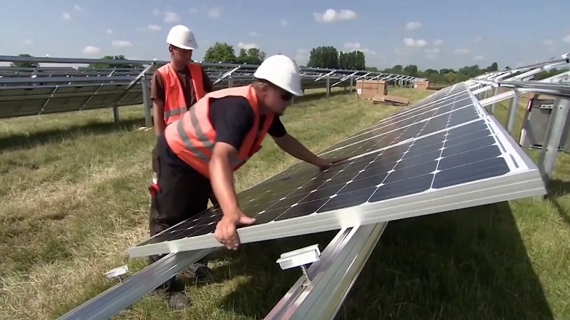