Hydrogen has been used in industry at large scales for over 50 years, primarily in petroleum refining and ammonia production^1,2. Recent growth in industrial demand for H₂ can be attributed to methanol synthesis and the direct reduction of iron (DRI; see Supplementary Note 7 for nomenclature list)^3,4. In these cases, the feedstock is syngas, a mixture of H₂ and carbon monoxide, rather than pure H₂. Switching these processes from syngas produced from fossil fuels to pure H₂ from renewable resources requires modifications to the methanol and DRI processes, but such modifications are a relatively low-hanging fruit for decarbonizing industry as they target gaseous feedstocks rather than the more complex electrification of processes.

Nearly half of global H₂ is produced from natural gas, 22% from petroleum, 27% from coal, and only 4% from electrolysis, with total emissions of 830 million metric tonnes of CO₂e per year (CO₂e, CO₂ equivalence)^5,6. To serve large industry applications with renewable H₂, it is necessary to reliably deliver large quantities of H₂ year-round at a carbon intensity of 4 kg-CO₂e/kg-H₂ or less. Fossil-based H₂ can be produced at a very high capacity factor, while capacity factors for utility-scale wind and solar in the U.S. are improving but relatively low, at ~36% and ~27%, respectively^7,8. Such capacity factors can be improved through a number of methods including combining wind and solar, but only energy storage or hydrogen storage can truly address the issue of renewable resource intermittency. In an onsite H₂ production scenario, electrolyzers, powered by an appropriately sized co-located wind and solar facility, supply H₂ to the industrial process in real-time while supplying excess H₂ to a storage system during times of renewable surplus⁹. During times of scarcity, the H₂ storage system ensures the industry end user has adequate H₂. Industries are beginning to implement clean hydrogen to reduce emissions^10,11,12, but many hurdles remain to deployment at scale. For the iron and steel sector, some planned or scheduled turndown is possible, but the penalty of unplanned or extended duration DRI process shutdowns (e.g., from a lack of available renewable energy) can cost millions of dollars per day. Another approach is to turn down steel or ammonia production (e.g. companies such as Haldor-Topsoe and Casale are working on more dynamic plant operation for ammonia plants); however, this still leads to an underutilization of the installed production equipment. While long duration H₂ storage can increase productivity, careful sizing of the H₂ storage system is needed to ensure reliable and economical H₂ provision.

Numerous reviews of aboveground and underground H₂ storage systems have advanced the understanding of the portfolio of available technologies and their technical maturity^{13,14,15,16,17,18}. The suitability of such technologies for storing hundreds or even thousands of tonnes of H₂ has not been well established, largely due to a lack of data on the real-world requirements for hourly and seasonal storage in such applications. However, there is consensus that compressed buried pipes and cryogenic liquid storage will not be able to meet cost or size targets for gigawatt (GW)-scale storage (see Supplementary Note 4). GreenHEART¹⁹, a software recently developed by researchers at the National Laboratories to simulate wind- and solar-powered H₂ production and transportation in the U.S., addresses the data gap on H₂ storage requirements. Other materials for H₂ storage are under development, including metal hydrides and adsorbents; however, we exclude these materials due to their current material cost, the need for temperature and pressure regulation during storage, the sheer magnitude of storage vessels and balance of plant required, and their relatively slow charging rates. Pipelines can offer some storage, particularly in very large (32” diameter) pipes, but cannot solve the issue of renewable seasonality, and are therefore excluded from this study. Finally, while ammonia and methanol are expected to serve a role in bulk H₂ transportation, they are limited in that the carrier gas must be generated onsite or recovered, methanol is tied to CO₂ capture cost and policies, and ammonia cracking remains highly energy intensive.

A wealth of research has focused on aromatic benzene-based hydrocarbon carrier materials such as methylcyclohexane (MCH, C₇H₁₄)^16,20. Hydrogenation of toluene (TOL, C₇H₈) to MCH is a commercial process, while dehydrogenation of MCH is still under development. The TOL/MCH system has been recently demonstrated, pre-commercially, as a global H₂ supply chain by the Chiyoda Corporation²¹. Limitations discussed in previous reviews include the use of a sulfur-platinum (Pt)/AlO₃ catalyst, which can cause corrosion of industrial equipment and somewhat low selectivity, but whether these limitations affect the ability to meet technical requirements in a stationary application is not clear.

In this work, we present estimates of the necessary storage capacity to smooth renewable H₂ delivery from dedicated wind and solar facilities powering industry-scale (i.e., 1-GW-scale) electrolyzers. We model and benchmark the performance of a liquid organic H₂ carrier (LOHC) that can be scaled and cycled for stationary storage and can store H₂ for long periods at high densities. We use TOL to MCH as a model material to represent LOHC systems, which take gaseous H₂ and convert it to a stable liquid for storage²². We compare the performance of this stationary LOHC with cryogenic liquid, compressed gas buried pipe (100 bar), lined rock caverns (LRC) and salt cavern storage, following the method of Papadias and Ahluwalia, discussed in Supplementary Note 4^22,23,24. Cost drivers and opportunities for cost reduction are identified, and scaling equations are provided, as the methodology employed in this study required use of a high-speed computing cluster at the National Renewable Energy Laboratory (NREL). These equations are detailed in this paper to facilitate adoption by the research community and can be used to evaluate other materials using the GreenHEART model. Based on the locations evaluated, significant amounts of H₂ storage (1457–19,837 tonnes) are necessary to smooth annual supply from the electrolyzers, highlighting the importance of developing low-cost underground storage facilities where available. At the same time, the expected added cost for H₂ end-users (ACEU) of aboveground TOL/MCH storage falls below a threshold target¹¹ of 0.7 $/kg-H₂ in many key industrial regions, potentially meeting delivery cost requirements as long as the cost of H₂ production can be lowered to $1/kg-H₂ in the near term through policy incentives.

In this section, we present results for the TOL/MCH storage systems we developed in Aspen Plus software based on renewable power profiles at select locations in the United States. Hourly production data for 50,052 hypothetical electrolyzer facilities were generated using GreenHEART¹⁹. The model first identifies combinations of wind, solar, and batteries to generate least-cost power. The resulting renewable power profiles are coupled with a 1-GW-scale electrolyzer facility model. (Calculations are shown in the Methods section and Supplementary Notes 1−3.)

Industry end users will have varying target design capacities that may require significantly larger systems than what is considered here for a 1-GW-scale dedicated renewable generation system. We include one such example, located in Southwest Texas, noting the electrolyzer-to-storage system sizes necessary to serve an industrial end user at 200 tonnes per day (TPD). This daily consumption target was set based on the approximate threshold where steam methane reforming (SMR) is no longer cost competitive and where a steel facility would still produce large amounts of steel (>1 million tonnes steel per year)¹¹.

Storage design and key assumptions

Key assumptions are that, first, H₂ production from the electrolyzers to the end user varies from zero, when power goes below the turndown ratio, to the beginning-of-life nameplate capacity of 18,698 kg-H₂/hour or 449 metric TPD. Second, H₂ from the electrolyzers flows directly to the end user until the facility’s H₂ demand is fully met; thereafter, any surplus (i.e., otherwise-curtailed H₂) is sent to the storage facility. As such, we prioritize storing all otherwise-curtailed hydrogen. Throughout the year there will be hours when the storage is running below its designed delivery capacity, but on an annual basis the quantity of stored H₂ is equal to the facility’s annual demand for stored H₂. The remaining stored H₂ at the end of a year becomes the new start fill level (Fig. 1). Over the course of a year, a peak in stored H₂ can be identified based on the net amount of MCH in the storage system, as was determined by evaluating changes in storage level over the course of a year at an hourly granularity (Fig. 1). These assumptions dictate the size and operation of the hydrogenation unit, storage tanks, and dehydrogenation unit.

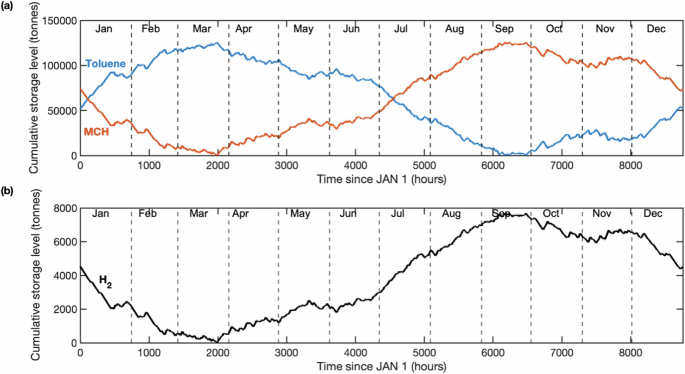
a Cumulative liquid storage of toluene versus methylcyclohexane over a sample year for a location with the median national levelized cost of storage of $1.84/kg-H₂. b Stored H₂, which is equivalent to surplus or otherwise-curtailed H₂.

Full size image

Performance for industry in Southwest Texas

In the following section we dive deeper into a potential industrial facility in Southwest Texas, which is a promising location for DRI steel production. The Southwest Texas electrolyzer facility produced 200 TPD at power nameplate capacity of 1.6 GW and capacity factor of 30%. For reference, five other locations evaluated for 1 million tonne steel facilities in the GreenHEART model ranged from 0.96 to 1.52 GW¹⁹. The levelized cost of storage (LCOS) when using the TOL/MCH model developed in this study at the exemplary Texas site is $2.17/kg-H₂ (Fig. 2). Capital costs (CAPEX) account for more than 50% of LCOS, with the dehydrogenation plant contributing significantly (22%); methods for lowering upfront CAPEX are detailed in Supplementary Note 1. Natural gas contributes $0.19/kg-H₂ and 80% of greenhouse gas emissions associated with consumables (Table 1). The liquid storage accounts for 13% of the LCOS, with the majority of that cost attributed to the first fill of TOL (treated as CAPEX). Greenhouse gas emissions from the storage system (3.77 kg-CO₂e/kg-H₂-stored) stem from TOL and catalyst first fill and replacement, along with consumption of electricity (Texas grid) and natural gas (Supplementary Note 2). Leveraging renewable electricity rather than the Texas grid could lower indirect upstream emissions (i.e., those not directly produced from storage system processes) from 1.44 to 1.00 kg-CO₂e/kg-H₂-stored. Methods to lower natural gas consumption offer the most significant means of driving down carbon intensity (CI).

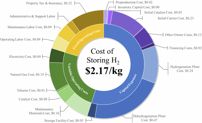
Breakdown of levelized cost of storage in a case where the storage facility is serving a 200 tonnes per day end user. Hydrogen storage size is 3156 tonnes.

Full size image

At this location about one quarter of H₂ production required storage, and the resulting ACEU would be $0.54/kg-H₂. Based on recent assessments of market liftoff for H₂, under policy incentives that drive H₂ production costs down to $1/kg-H₂, this added cost would meet the $1.7/kg-H₂ price point requirement of iron and steel facilities¹¹ but may lead to some price increase for ammonia compared with fossil-based production¹⁹. When compared with other large-scale H₂ storage technologies (Supplementary Fig. 7), we find the carrier system outcompetes gaseous buried pipes and cryogenic liquid H₂, but not geologic solutions such as LRC and salt caverns²². While green at 1.44 kg-CO₂e/kg-H₂-delivered, this example supply of H₂ from dedicated renewables would not meet the required CI to qualify for the full United States Internal Revenue Service Production Tax Credits (PTC), which are likely necessary for achieving a $1/kg-H₂ production cost, unless the emissions from storage are excluded.

Performance for storing otherwise-curtailed H₂

Returning to our discussion of storage capacity for 1-GW-scale electrolyzer facilities, we estimate production and storage costs based on least-cost dedicated wind and solar electricity generation for specific locations across the contiguous United States. The capacity factor of electrolyzers ranges from 17.8% to 78%, with the lower end representing locations that produce very little H₂. The larger the capacity factor, the less a facility relies on H₂ from the storage to meet its average daily supply. As can be seen from Supplementary Fig. 3a, achieving a steady supply of H₂ to an end user could require anywhere from 1457–19,837 tonnes of storage. The distribution in LCOS is centered around a median of $1.84/kg-H₂, with a minimum of $1.31/kg-H₂ and maximum of $2.68/kg-H₂ at the national level (Fig. 3). Even with storage as a means of capturing surplus, the average delivered H₂ could be as low as 87 TPD or as high as 350 TPD (Supplementary Fig. 3d), with storage representing between 46 to 96 TPD of additional capacity, or 16% added capacity on average (Fig. 4). As such, many sites evaluated would require electrolyzers larger than 1 GW to serve a 200 TPD end user (e.g., medium-sized steel facility). In the approach presented in this work, storage system nameplate capacities are determined based on a set of rules, while capacity factors reflect actual operation and time of use over the course of a year. While the size of the hydrogenation system predictably increases with solar fraction, other key parameters such as the storage size and annual usage of the storage system (Supplementary Fig. 3b) cannot be estimated without evaluating temporal data for a location’s renewable profile, as conducted in this study.

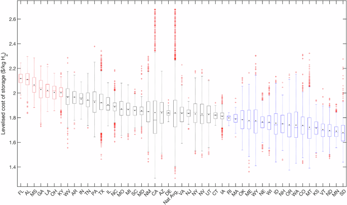
Variations reflect impact of hourly renewable power profiles on LCOS. Abbreviations of states listed in Supplementary Note 7.

Full size image

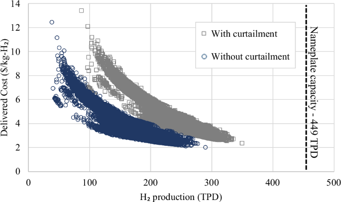
Storage is sized to capture all curtailment, allowing a facility to produce hydrogen at an average daily capacity closer to the electrolyzer facility nameplate capacity.

Full size image

There is a clear positive trend between the size of the dehydrogenation facility, its operating time, and LCOS, but the stronger predictor of LCOS is maximum storage capacity. Overnight capital costs contribute 40–50% to LCOS at the 20 cheapest sites and ~70% to LCOS at the 20 costliest sites (Supplementary Fig. 9). Furthermore, we find, the costlier sites follow a smooth sine curve in tank fill level, with hydrogenation occurring from Mar until Sep and dehydrogenation occurring from Oct until Feb (Supplementary Fig. 10). This two-mode profile results in a larger maximum storage capacity due to a surplus of otherwise-curtailed H₂ during summer and a shortage of H₂ production from the electrolyzer during winter. Cheaper sites tend to have several large hydrogenation and dehydrogenation events year-round, thus lowering the need for large storage despite processing a similar amount of H₂ as the costlier sites. Furthermore, there is a clear inverse trend between the total annual H₂ delivered to an end user and the delivered cost of H₂ (Fig. 4), which constitutes the cost of producing H₂ (Supplementary Fig. 11), plus the ACEU which is weighted based on the amount of H₂ stored (Supplementary Fig. 13).

Regional variations in H₂ production, storage, and delivered cost

Storage costs have a relatively small spread but are highest on average in Central California due to high solar dependence, followed by the Southeast, the Rustbelt, and Southwest Texas, and cheapest in the North and Midwest (Fig. 3 mapped in Fig. 5a). The largest dehydrogenation (Fig. 6) and hydrogenation systems (Supplementary Fig. 12) are also in distinct regions, with notably high dehydrogenation capacities possible in the Midwest at moderate LCOS. There are dramatic variations in production costs across the country (Supplementary Fig. 11), with no locations that can achieve $1/kg-H₂ without policy incentives in the short term. When deriving the ACEU (Fig. 5b), the cost impact of storage on the delivered price of H₂ mapped in Fig. 7 is clearer. While salt cavern storage may increase delivered cost by $0.07–0.22/kg-H₂ depending on annual use, we find TOL/MCH systems could also offer sub-$1 increases to delivered cost, as low as $0.35/kg-H₂.

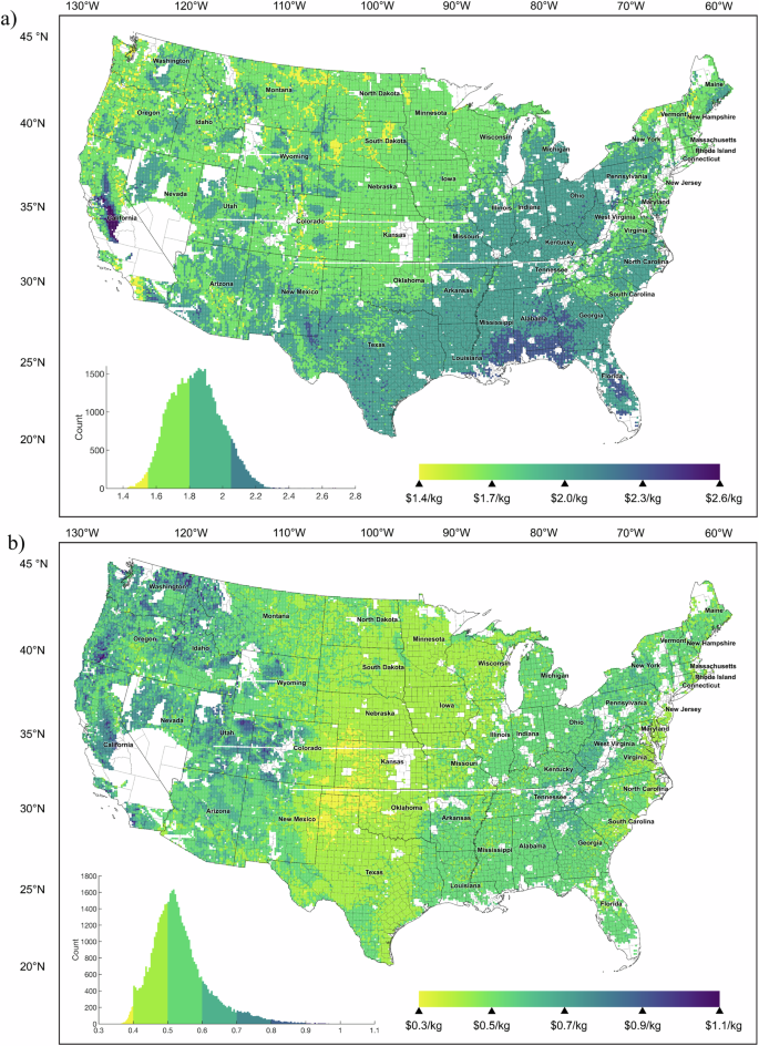
a Levelized cost of storage (LCOS) for least-cost wind- and solar-based H₂ production sites. b Additional cost to end user (ACEU) that would increase the cost of produced H₂ depending on the quantity of H₂ stored.

Full size image

Locations included with a dehydrogenation capacity greater than 200 TPD.

Full size image

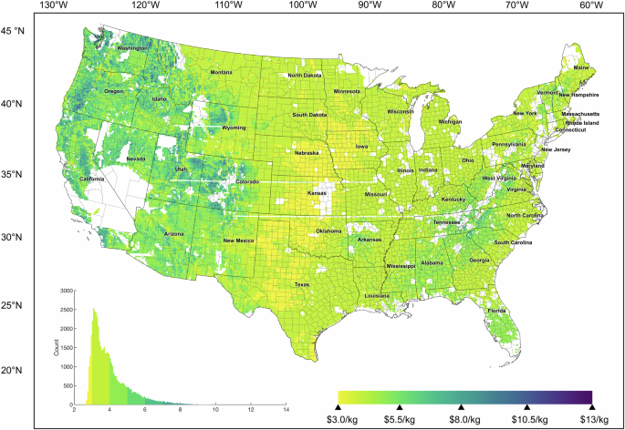
Delivered cost is the sum of the levelized cost of H₂ production estimated in the GreenHEART model assuming no policy incentives and the additional cost to end user resulting from the storage system based on annual use (ACEU).

Full size image

In this section, we present values for several important performance metrics other than cost and carbon emissions, including storage duration, energy density, specific energy, efficiency, purity, and charge and discharge rate for the storage system facility. These values are based on literature review, process design and models, technoeconomic analysis, and evaluation of industry needs. An evaluation of safety considerations was provided by the United States Department of Energy Hydrogen Safety Panel, included in Supplementary Note 5. While land footprint is challenging to estimate for emerging storage systems, we estimate that even when considering storage tank safety requirements, the TOL/MCH storage system will have a 4x smaller land footprint (1.38 hectares) than 350 bar compressed gas.

We assume TOL has a shelf life of 30 years based on personal correspondence with Chiyoda Corporation and thus meets storage duration requirements. Multiple days of H₂ storage are possible and economic, but increasing maximum storage capacity dramatically increases upfront CAPEX and should be minimized. The TOL/MCH material offers efficient recovery of H₂ at relatively mild conditions, improving overall usable storage capacity. In comparison to other LOHC materials, TOL/MCH has high conversion, selectivity, and catalyst stability and is one of the most mature systems in terms of market development. However, TOL/MCH produces a lower energy density and specific energy relative to other mature liquid organic H₂ carriers and requires excess H₂ during hydrogenation and co-feeding of H₂ during dehydrogenation (Table 2). The system operates with a low-pressure dehydrogenation (output H₂ is at 1.5 bar), while the higher vapor pressure of TOL and MCH make recovery costlier than some carriers such as dibenzyltoluene. Furthermore, the reactions occur at high temperatures and in the vapor phase with a high reaction enthalpy, requiring the burning of natural gas and warranting careful control of temperature control via methods such as steam condensation/evaporation. Despite the promise of LOHC as a solution for regions where large-scale, low-cost salt caverns are not available, we find the system has very large capital costs associated with process equipment and first fills of TOL (Table 2). The price volatility of the hydrogenation Ni catalyst and possibly TOL (Supplementary Note 1), and dependence on dehydrogenation Pt catalyst, may be a concern and supply chains will impact carbon intensity.

Based on our total plant energy balance (not including losses during the generation of grid electricity), we estimate the energy efficiency of H₂ storage and release. For our case location, while H₂ recovery is 99.8%, the energy efficiency of the storage system is moderate (60%), with 240,117 MWh/year consumed compared with what is stored in the H₂ (e.g., 607,200 MWh, assuming a 33 kWh/kg lower heating value). Measures for reducing upfront CAPEX and improving energy efficiency are discussed in Supplementary Note 1. Systems that reduce natural gas and TOL consumption will achieve substantially improved CI as well. This is possible by reducing the operation of the dehydrogenation facility (which however is directly coupled to the amount of H₂ stored) or finding means of reducing heat consumption (e.g., by thermally coupling hydrogenation with dehydrogenation, which could be achieved by coupling the storage system to a steam cycle) and TOL losses. At the same time, conversion efficiency and kinetics are more important than achieving a lower operating temperature in terms of lowering costs, but coking resistant catalysts are essential (see Methods). We find that using H₂ for heating is not a viable option. There would be advantages in lowering the life cycle greenhouse gas emissions of the storage system if renewable H₂ were used in place of natural gas. However, more than 30% of the stored H₂ would be consumed to operate the dehydrogenation system and the effects on key technical requirements (e.g., round trip efficiency and on cost due to oversizing the power and electrolyzer system) are non-viable. The proposed use of industrial waste heat comes with the nontrivial challenge of coupling intermittent heat demand with a heat source. We encourage research on the electrification of dehydrogenation, provided that a low-carbon source of electricity is available.

Pretreatment requirements are set based on discussions with industrial stakeholders. We estimate that H₂ leaving the storage unit will require compression of at least 3 bars for piping into an industrial facility. In the case of an iron and steel facility, heating is required prior to entering the DRI. Some TOL in the DRI is actually advantageous as it can add carbon to the iron, which is desirable in steelmaking.

The size of both hydrogenation and dehydrogenation reactors is set based on reaction rates and reactor kinetics which are poorly described in literature, and it is possible that a gaseous H₂ ballast is necessary for the dehydrogenation system (see Methods). Storage of compressed H₂, even for small ballasts, will introduce more challenging safety concerns (Supplementary Note 5). Understanding how to operate the storage system to meet transient renewable power and the effect on equipment needs is an important research area. Based on our design of the storage system, where heat is rejected via the TOL steam drum, we always have sufficient TOL vapor available to ramp up hydrogenation as soon as extra H₂ becomes available. Of course, this does not completely eliminate concerns regarding the ramp rate, but with this design modification we expect this process to be load following, without the need of any gaseous H₂ buffer storage. Dehydrogenation is dictated by the ability to generate steam, and as such, this configuration would be similar to once-through boilers, thus ramping around 8–10% per minute. Finally, due to reliability issues, a facility must be designed for anticipated transients from renewable power. This includes a backup scenario where 100% H₂ is supplied from the storage unit for multiple days, which the storage systems in this study achieve (i.e., max storage divided by dehydrogenation capacity).

Widespread deployment of wind- and solar-powered H₂ generation at industrial scales will require aboveground storage solutions for seasonal and daily storage of H₂, due to the limited near-term availability of solutions for bulk H₂ storage and transport, such as salt caverns, LRC, and large pipelines. In particular, there is no H₂ pipeline system comparable to the extensive United States natural gas pipeline system that would conveniently distribute H₂ from where it is generated to where it is used. Until there is such a H₂ pipeline system, onsite H₂ production and storage systems based on H₂ carrier materials are one solution. However, little has been reported regarding their technical, economic, or health and safety viability for bringing industry-scale levels of renewable power and H₂ production into the economy.

The ability of an aboveground H₂ storage system to hit industry targets for delivered renewable power despite variations in renewable wind-solar generation profiles in the United States is encouraging and warrants the serious consideration of H₂ materials for seasonal storage and industrial applications. Large-scale seasonal storage and industrial applications require thousands of tonnes of hydrogen storage. This scale of storage has so far only been demonstrated as cost effective in underground hydrogen systems, but these systems are limited in their development and physical distribution. Costs for buried, compressed-gas systems in the form of underground pipes are astronomical and will not enable low-cost hydrogen to enter the market.

In this work, we evaluate a carrier that can cycle and that meets many technical and cost targets for industry. The analysis framework presented herein can be applied to other LOHC storage technologies as it translates renewable generation into electrolyzer operation, which is then translated into size and operational hours for storage, hydrogenation, and dehydrogenation. We find that thanks to the storage of otherwise-curtailed H₂, 1-GW wind-based electrolyzer plants can offer steady supply of H₂ between 80 and 350 tonnes per day, corresponding to electrolyzer capacities between 17.8 and 78% (national median, 56%) We find a national median LCOS of $1.84/kg-H₂ with minimal distribution, but marked variation in the final delivered cost of hydrogen to end users from $2.02 to $13.40/kg-H₂ (Fig. 7). We encourage the application of this methodology for analyzing H₂ storage including equipment scaling factors and system cost scaling equations, which are common methodologies used in chemical engineering, to reduce computational intensity and expedite the screening of storage technologies across a wide range of diverse and complex hydrogen production and end use applications.

Supply chain model

The 50,052 locations were chosen from NREL’s reV model²⁵ and exclude areas with wind siting ordinances²⁶. Locations without data have restrictions on wind turbine deployment, including military sites and protected land²⁷. No site-specific land restrictions were included in this analysis. For each site, the Hybrid Optimization Performance Platform (HOPP) software simulates the hourly performance of the off-grid hybrid renewable energy plant, consisting of wind and solar assets²⁸. The wind and solar capacities are selected through a parametric sweep. Wind capacities of 228 MW, 672 MW, 900 MW, 1350 MW, and 1572 MW are swept. For each wind capacity, we then sweep solar capacities of 5 MW, 125 MW, 375 MW, 500 MW, 750 MW, and 875 MW. Out of the 25 plant capacity combinations, the design resulting in the lowest cost of produced hydrogen is selected as the final design.

Site-specific wind resource data is pulled from the WIND Toolkit²⁹ for a hub height of 115 m, corresponding to the land-based-wind 6 MW turbine. The hourly resource data, turbine power coefficient (Cp) curve, and total wind farm capacity are input to the PySAM default WindPower module, which then simulates the hourly wind farm power production. Hourly solar resource data is pulled from the National Solar Resource Database (NSRDB). Solar resource data and the DC nameplate capacity of the photovoltaic (PV) system are input to the PySAM PvWattsv8 module, which simulates the hourly solar system power³⁰.

The wind and solar generation profiles are summed together and input to the GreenHEART electrolyzer system supervisory control model¹⁹. The electrolyzer system is rated at 1 GW, comprised of 25 stacks with balance of plant rated at 40 MW³¹. The electrolyzer stack is modeled at the cell level using first-principles equations and includes degradation and dynamic losses in HOPP. The supervisory controller does a “basic-even-power-split” control method to distribute power amongst the stacks. The output hydrogen production is then input into the Production Financial Analysis Scenario Tool (ProFAST) to calculate production cost³². It is expected that the electrolyzers will be run at some small fraction (5–15%) of rated power during times of scarcity or turndown, and therefore will always supply some hydrogen to the end use. However, given the uncertainty around how electrolyzers run solely on dedicated renewable power will operate to meet lower sustainable operating limits, we conservatively assume the hydrogen storage system must be able to fully serve the end user during periods of turndown and size it accordingly.

Annual hydrogen production from the electrolyzers is determined by taking the sum of hourly production (P_i). This value divided by 8760 hours gives an estimate of average hourly hydrogen production (P_avg), which is equivalent to the end use design capacity. We fix P_avg in our case study and estimate the necessary size of all other equipment for the Southwest Texas renewable profile, while in the national sweep we only fix electrolyzer size (P_nameplate). In our base case, the storage facility is designed to capture 100% of otherwise-curtailed hydrogen. In Eq. (1), we estimate otherwise-curtailed hydrogen as all hydrogen generated in an hour where hourly production is above P_avg.

where i is the hour of the year, and AS is the total amount of hydrogen directed to the storage system. The hydrogenation facility is sized to allow for a peak hydrogen storage rate (HC) noted in Eq. (2); however, this peak hydrogen storage rate will only be seen during peak electricity generation from wind and solar and in practice much smaller flow rates will be observed on most days. Locations with limited renewable power generation will have a large HC. In our study of seasonal storage, P_nameplate is constant for the 1 GW scale electrolyzer, while in our study of industrial-scale production P_avg is always fixed at 200 TPD.

Importantly, the total quantity of H₂ flowing into the storage facility over the course of a year does not determine the quantity of TOL required for storage. Rather, it is the maximum consecutive quantity of H₂ stored, with lowest frequency of use/discharge, and equivalent quantity of TOL required for converting the H₂ to MCH for storage, that sets this maximum storage capacity (MS) (Supplementary Fig. 3a). In other words, H₂ may enter the storage system and may be used in following hours and days during shortages of renewable power. However, if the H₂ needs to be stored over months, MCH will accumulate in the storage tank. It is critical to ensure this peak is also large enough to meet the end user’s required daily demand for H₂, which we set equal to ({{{{rm{P}}}}}_{{{{rm{avg}}}}}). Thus far, we have derived a method for obtaining the hydrogenation capacity, the maximum storage size, the operational hours and flow of H₂ into the storage system. The final parameter necessary for coupling the electrolyzer profile to the storage system is the dehydrogenation capacity (DC). This is simply equal to the average hourly production rate as noted in Eq. (3), as we assume an end user that requires a consistent supply of hydrogen. The quantity discharged from the storage system is determined in Eq. (4).

We acknowledge electrolyzers will likely operate at some capacity during turndown to improve their longevity, and will rarely produce zero quantities of hydrogen. As such, our analysis can be considered a conservative estimate that oversizes all systems by some percentage. Furthermore, our approach does not force the storage facility to completely empty by the end of the year, as our priority is to meet all periods where there is a shortage of power. We therefore will have some oversizing of the quantity of TOL required.

MCH/TOL process model

Conversion of hydrogen and TOL to MCH for storage, and MCH to TOL with recovery of the hydrogen, is influenced by several key operation decisions. First, hydrogenation of TOL occurs over a nickel-based catalyst and full conversion is thermodynamically favored at low temperatures, high pressures, and excess hydrogen (described using a hydrogen-to-TOL ratio) (Supplementary Fig. 1). However, to achieve appreciable reaction rates, it is desirable to operate the reactor at higher temperatures. Carbon deposition is a concern with hydrocarbon feedstocks over nickel catalysts, which can be minimized by supplying sufficient excess hydrogen. Dehydrogenation of MCH occurs over a Pt-based catalyst and full conversion is thermodynamically favored at high temperatures and low pressures (Supplementary Fig. 2). An upper practical operating temperature exists to avoid undesirable side reactions that would decompose the carrier material and carbon deposition. As such, thermal management of both reactors is critical for longtime operation. Conversion from literature studies is high (>98%) and suggests nearly 100% selectivity²². Due to the high cost of the carrier material, toluene, it is important to have high separation and recovery efficiencies of TOL from the hydrogen product stream regardless of the application’s requirements. In our baseline model, the H₂ stream produced from the dehydrogenation of the MCH is cooled to below −30 °C to condense residual TOL for recycling. While this chilling process is energy intensive, the compression stage is significantly more so.

In order to develop a process for modeling the TOL/MCH system across many locations, we started by constructing a process model in Aspen Plus at a relevant industrial scale. Previous work by several of the authors developed a process model for an TOL/MCH system where the hydrogenation and dehydrogenation facilities were decoupled (i.e., not co-located) to support the transport of hydrogen via ships using TOL as carrier. Ships holding TOL/MCH tanks would fuel and deliver hydrogen, respectively^13,14. Alterations to this transportation system were made in the balance-of-plant and heat integration, making this technology more applicable for stationary H₂ storage where hydrogenation and dehydrogenation systems are co-located with an end user. The dehydrogenation capacity was fixed at 200 TPD or 8333 kg H₂ per hour. The hydrogenation (475 metric tonnes H₂ per day) and storage capacities were derived from the selection of one location in Southwest Texas with favorable wind and solar to reduce the size of storage and where there is a presence of direct iron reduction activities. (Later we will discuss the scaling methodology to make this model applicable to any site in the US).

Toluene hydrogenation is a strongly exothermic reaction and is conducted in a tubular reactor (1870 tubes, 5 meter length, 5 centimeter diameter) with catalyst pellets on the tube side. The shell side acts as evaporator for the feed TOL, which provides a tight temperature control of the reactor (Fig. 8). The actual heat rejection occurs in a vapor condensation loop via an air-cooled exchanger. Hydrogen (added in excess) is pre-heated against the reactor outlet gas before being mixed with vaporized TOL and fed into the reactor at 210 °C. The reactor is operated at ~10 bar with an outlet temperature of 240 °C, whereby the peak temperature in the reactor is ~335 °C. The reactor is modeled as a plug flow reactor using experimental reaction rate expressions under consideration of pellet diffusion limitations³³. Using a kinetic reactor model provides the necessary information for reactor sizing and catalyst requirement. Excess hydrogen and MCH vapor are cooled to 45 °C and separated, and the excess hydrogen (and ~1.7 mol-% MCH which remains in the gas phase) is recycled to achieve a H₂/C₇H₈ ratio of 4, resulting in a 99.9% TOL conversion. Due to the high selectivity of this reaction³³, no side reactions are considered in the simulation. We allow for a 1.5 atm pressure drop across the reactor, with additional pressure drops accounted for in heat exchangers and separator. After the initial separation at elevated pressure, the liquid product is depressurized for storage in ambient pressure tanks. Depressurization of the liquid leads to further H₂ degassing and the tail gas is cooled to −30 °C to recover any degassed carrier before flaring the low pressure, H₂-rich tail gas. Cooling the tail gas to sub-ambient temperatures is achieved via a refrigeration cycle, which is shared with the dehydrogenation system³³.

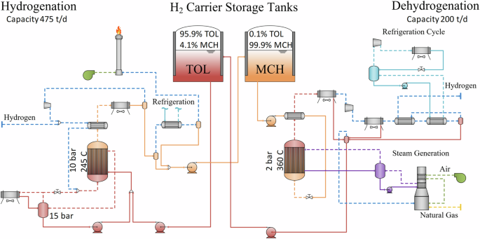
Process used to generate the Aspen Plus model. Analysis assumes H₂ storage is co-located with the H₂ from PEM electrolysis and an end use application.

Full size image

The MCH dehydrogenation system starts by pumping MCH from a storage tank to a reactor at 50 bar (Fig. 8). This pressure is above the critical pressure of MCH and allows for more efficient pre-heating against the reactor outlet stream and overall heat recuperation in the dehydrogenation system. The MCH is preheated to 310 °C, but is throttled prior to entering the reactor to 3 bar resulting in a gas inlet temperature of ~240 °C. The MCH dehydrogenation reactor is a tubular reactor consisting of 4500 tubes (5 m length, 5 cm diameter), more than double the amount of tubes at less than half of the capacity of the hydrogenation system. Kinetic rate expressions are used to determine performance and reactor size³⁴. Due to the endothermic nature of the dehydrogenation reaction, steam condensation is used for heat addition, which keeps the temperature above 340 °C for most parts of the reactor. The reactor outlet temperature is kept below 360 °C. Tight temperature control of the reactor is desirable, and using condensation rather than a conventional single-phase heat exchanger has advantages with respect to temperature control as well as higher heat transfer coefficients. Steam is an ideal heat transfer fluid for these purposes, as it has a high latent heat and avoids degradation problems of alternative heat transfer fluids. Furthermore, it provides integration advantages with other industries in the future. We note condensate circulation/pumping at 350 °C may present a challenge and requires high-temperature pumps that are only offered by a small number of vendors. Conversion under these conditions is 95.9% with an H₂/TOL ratio of 3 (stochiometric mixture). No side reactions were considered, as reactions are very selective to the preferred product²². The challenge of dehydrogenation is that large amounts of catalyst are required as the product is a stochiometric mixture, which also increases the risk of carbon deposition compared to hydrogenation. Hydrogen and TOL exit the reactor and are compressed upstream of the cryocooling unit to achieve 99.9% recovery of TOL/MCH. Condensed TOL is depressurized and pumped back into the storage tank. Finally, the H₂ is compressed to 3 bar, the pressure necessary for flow in pipes to a co-located industrial end user. We estimate about 230 ppm (mole basis) concentration of TOL and MCH in the H₂ stream exiting the storage system. Toluene makeup is calculated to be 0.07% due to hydrogenation and dehydrogenation losses related to degassing during depressurization of the liquid carrier.

The storage system runs on electricity (1.24 kWh/kg-H₂) and natural gas; the electricity may come from the renewable generation plant, but is represented as purchased industrial electricity cost in this study. Heat demand is estimated at 11.37 kWh/kg-H₂, while heat rejection is estimated at 6.36 kWh/kg-H₂. Chiller load is estimated at 0.16 kWh/kg-H₂. Our results are similar to the Chiyoda design and Argonne National Laboratory (ANL) designs, differing primarily in our selection of reactor operating conditions²², except for the chiller load which we reduce by more than half through design changes noted previously. The ΔH for the dehydrogenation process is 68.3 kJ/mol-H₂ (9.4 kWh/kg-H₂). Waste heat may be available for recovery from certain industrial processes; however, after careful evaluation it was determined that not much heat is available from a DRI system¹¹. Furthermore, the intermittent use of heat to power dehydrogenation makes coupling a challenge. Co-locating these H₂ storage systems at industrial parks with steam infrastructure with high-pressure steam would be an obvious advantage and reduce CAPEX and OPEX costs¹¹. However, for this study we assume the storage system uses natural gas for steam generation. To understand the sensitivity of our model to some of the design decisions made for the storage system, we compared our design to a second process model developed in Aspen Plus adhering to more conservative design parameters reported in literature (i.e., Chiyoda)^21,22. We estimate that with our advanced design, a ~ 15% lower LCOS can be achieved.

Future research on catalysts and system integration are needed to advance the development of this technology. The development of intrinsic reaction rates that cover the entire operating range encountered in this system are seen as the current limiting step to scaling this system. Intrinsic reaction rates are needed on both the hydrogenation and dehydrogenation sides. Access to reliable intrinsic rate equations is essential to catalyst pellet scale-up and maximizing catalyst effectiveness (equivalent to minimizing raw material use). Moreover, this information is critical to the development of effective reactor designs, e.g., the avoidance of hotspots, which are problematic in these systems due to the risk of carbon deposition. Congruent with this effort, it is important to understand the impact of varying operating conditions on side reactions and how to effectively remove or add heat to the reactors. Thereafter, dynamic simulation studies are needed to validate system dynamics (response behavior) and controls.

Financial analysis

The basis for the economic analysis is the year 2024. The LCOS is evaluated over an assumed 30-year plant operational period with a capital expenditure period of three years (33 years total). The total overnight cost is assumed to be 100% depreciable over 20 years at a 150% declining balance³⁵. After-tax weighted average cost of capital for an investor-owned utility with 55% debt financing is 4.73% (real)³⁵. Tax rates are 21% (federal) and 6% (state)³⁵. This financing structure results in a capital charge factor (CCF) of 0.0710. Equation (5) can be used to determine the LCOS when annual storage (AS) is nonzero.

The LCOS represents the cost of feeding hydrogen into the storage system in the first year, calculated by considering factors such as the CCF, the total cost of building the facility (TOC), fixed and variable annual operating costs (OC_fix and OC_var), the hydrogen storage efficiency (e = 99.84%), and the expected annual quantity of hydrogen being stored at full capacity (AS). The cost seen by an end user can be taken as the cost of hydrogen delivered from the electrolyzers (production cost) and the cost of otherwise-curtailed hydrogen put into storage, weighted by annual quantities stored (ACEU) as see in Eq. (6). Naturally, the system cost for a given capacity will remain regardless of its frequency of use, and these equations are intended to represent operation with significant (10% or more) quantities of otherwise-curtailed hydrogen.

The TOC is the total overnight capital expenditure and includes the total plant cost (TPC) of the hydrogenation, dehydrogenation, and storage components, as well as pre-production costs, inventory capital, financing costs, land ($250,000/acre), and other owner’s costs. Capital costs estimates are based on Aspen Plus economic evaluation and values reported in literature (Supplementary Note 1).

Fixed operating costs (OC_fix) include property tax and insurance at 2% of the TPC, and operating labor. Operating labor for the integrated storage facility at the relevant scale is estimated at 100% capacity factor, with skilled operators paid at an hourly rate of $38.50, based on median salary for power plant operators. It is estimated that the operating labor burden accounts for 30% of the operating costs, and an additional 25% will be allocated for overhead expenses. Maintenance-related labor expenses are assumed to make up 35% of the maintenance costs, and administrative and support labor are assumed to be 25% of the combined operating and maintenance labor costs. Operators per shift are derived from Turton³⁶.

Variable operating costs (OC_var) such as maintenance expenses are dependent on the operation hours of the plant. Variable costs to consider include items like fuel (electricity and natural gas), toluene ($1089.43/tonne), and catalyst that are consumed. We assume a NiSat 310 52% nickel catalyst at $93.15/kg, and ATIS 2 L/SD platinum alumina catalyst at 1% Pt at $191.35/kg based on import data on Zauba. The price of Pt may be higher than the equivalent bulk value of $13,500/kg, but we find that adjusting to a spot price of $31,781/kg only increases levelized cost by one cent. Both catalysts are assumed to have a lifespan of six years. We assume a natural gas and electricity price for industrial consumers of $16.03 and $73.79/MWh respectively. A summary of the consumables used in the storage system is provided in Table 1 (for the analysis, all costs are escalated to the year 2024 using an annual escalation factor of 3%). We assume a life-cycle carbon intensity of consumables to estimate the carbon intensity of storage operation (refer to the Supplementary Note 2).

Scaling equations development

Each location considered has a distinct renewable energy profile, which lends itself to a unique set of requirements and pattern of use for the storage system and associated sizes of equipment involved. The equipment sizes are then assigned some ratio in comparison to the reference Aspen Plus system³⁷. Scaling factors for individual equipment components are supplied in Supplementary Note 1 along with capital costs, and scaled cost is estimated based on the reference case and year, adjusted to the scaled cost and scaled year (Supplementary Table 1). The LCOS for each location is computed using macros in Microsoft Excel. However, it is possible to quickly estimate the TOC, OC_var and OC_fix with minimal error and without a complex Excel model by generating scaling equations at the hydrogenation, dehydrogenation, and storage system levels. This approach significantly reduces computational cost and allows the broader research community to estimate the LCOS for any location with known hydrogen production profiles in the range of ~85–350 tonnes per day, at 17.5 to 55.5% of annual H₂ curtailed to the storage system. We derive constants in Eq. (7) by capturing the impact of hydrogenation capacity, dehydrogenation capacity, maximum storage capacity, and annual hydrogen curtailment stored on TOC, OC_var and OC_fix (see details in the ESI). Scaling equations were derived from linear interpolation across ranges in HC, DC, MS, and AS identified from the 50,052 locations. While not important at the final equation level, we allocated land cost fully to maximum storage and split labor equally between the hydrogenation and dehydrogenation facilities in the process of deriving scaling equations. Location-specific policy incentives, labor, land, feedstock and energy costs are not considered in our results, but are considered in the sensitivity analysis. Similarly, efficiency changes of the storage system due to scaling effects are not captured in this approach but are expected to be small. The scaling Eq. (7) is then used to reevaluate the LCOS of locations and absolute errors are evaluated in $2024USD.

where HC, DC are in tonnes per day while MS and AS are in tonnes, and e is a percentage.

Ranges in storage costs and capacities were used to develop scaling equations that reflect the influence of these parameters for TOC, OC_fix, and OC_var, which were ultimately used to derive the scaling Eq. (7) (Supplementary Table 2). We conducted an error analysis and found an error resulting in a LCOS difference of $0.03/kg-H₂ or less for the location’s evaluation (Supplementary Fig. 4), and an error greater than 2% at only the extreme minimum evaluated in Supplementary Table 2, which does not reflect any location identified.

The system modeled in the case study met the cost target for iron and steelmaking but represents a location and solar-to-wind ratio (69 to 31%) that minimizes storage requirements. We use the scaling equation to explore the LCOS for the iron and steel sector based on identified plausible ranges in hydrogenation capacity and annual storage (in effect, capacity factor of the electrolyzer) (Supplementary Fig. 5). The national sweep inputs also optimize with respect to wind and solar use prior to feeding into the storage scaling equation. As such, the power-to-storage supply chain is not optimized for least-cost delivered H₂ for the national locations, as we assume facilities will be designed for least-cost renewable power and hydrogen generation. For systems with hydrogenation capacity ranging from 80 to 400 tonnes, and with a fixed maximum storage size of 15 days (3000 tonnes) similar to the case study size, levelized costs of delivered H₂ are possible between $1.55–1.62/kg-H₂ for renewables with a capacity factor of 50%, while a system used only 1/10th of the year is likely to generate H₂ costing closer to $1.40–1.47/kg-H₂, all of which meet the cost requirements for steelmaking. However, when holding hydrogenation capacity constant and varying maximum storage size (1000 to 20,000 tonnes H₂), we find the cost of delivered H₂ could increase to $1.92/kg-H₂. This result suggests that the cost of significantly oversizing the storage system in relation to what might be necessary for a given location should be avoided. As the cost of producing H₂ decreases, the value of storing otherwise-curtailed H₂ decreases, and it may be more cost effective to oversize H₂ production than to pay for excess storage.

Like all storage technologies, facilities that do not leverage the storage facility have sitting capital and high LCOS that is independent of the annual usage of the storage facility. However, once sized, the annual storage may vary from year to year and the effect can be evaluated by the impact on the delivered cost (Supplementary Fig. 5). For example, facilities with maximum storage at or above 9750 tonnes H₂ may no longer achieve the $1.7/kg-H₂ delivery cost depending on use.