Saudi Arabia has set an ambitious target of generating at least 50% of its electricity from renewable sources under its Vision 2030. The Kingdom’s plan aligns with its commitment to diversify its oil-centric economy by exploring alternative fuels, including low-carbon hydrogen and ammonia¹. This transition mirrors global trends. For instance, the United States aims for 100% clean electricity by 2035 and has set a goal for net-zero emissions by 2050². Similarly, the EU has set a target to achieve a renewable energy share of 32% by 2030 with the potential aim to raise that target to 42.5%³. Saudi Arabia is especially poised to jump-start its clean energy sector given its abundance of solar⁴ and wind⁵ resources.

However, integrating renewable technologies poses considerable challenges concerning the reliability and resilience of the power system. The inherent intermittency of renewables requires that annual investment decisions carefully account for the variability of weather patterns to ensure that energy demand is consistently met. Whereas high-resolution weather data are now available at hourly timescales and spatial scales as small as a few kilometers, incorporating such data into optimization problems leads to computationally costly or intractable models.

Furthermore, the tight junctions between power and other sectors, such as water and heat, motivate taking an integrated sector-coupled (multi-sector) approach. Taking such an approach involves optimizing sectors simultaneously and allowing the exchange of information about demand and generation. Integrated energy systems modeling^{6,7,8,9,10,11,12,13,14} offers a comprehensive understanding of how various parts of the energy sector interact, resulting in more robust solutions than the independent optimization of each sector. Taking a multi-sector approach leverages opportunities for improved technology integration and economic efficiencies that are not apparent if the sectors are optimized independently.

A case-in-point concerns the nexus between water and power systems in water-scarce regions through energy-intensive desalination processes. Riera et al.¹⁵ found that co-optimizing the power and water sector allows the water sector to engage in demand-side management and reduce power demand during peak periods. Coordination of the capacities in power generation, energy storage, water desalination, water storage, and operations of the power and water systems resulted in cost reductions compared to the total cost of each system when optimized separately. Al-Mubarak and Conejo¹⁶ found similar results and highlighted that the coordinated scheduling of the power and water sectors results in lower costs.

By considering multiple interacting sectors, co-optimization compounds difficulties associated with considering fine-scale data. Numerous techniques have been proposed to reduce the size of the input data and the associated model complexity¹⁷. Spatially, data can be aggregated based on predefined political boundaries, such as states or provinces, using average or median weather conditions as representative values for these regions. An alternative approach involves segmenting a region into nodes based on similar climatic and demand profiles¹⁸; clustering algorithms have proven effective in these cases¹⁵.

Temporally, numerous techniques have emerged, including random sampling of periods, averaging periods (where average weather conditions and demands are considered), downsampling and segmentation, and feature-based merging—most notably, clustering¹⁹. Teichgraeber and Brandt²⁰ reviewed the impact of using various clustering techniques such as k-means, k-medoids, hierarchical, and k-shape methods.

Numerous studies have relied on clustering to capture the variability of renewable resources^{18,21,22,23,24,25,26,27}. However, clustering methods inherently smooth out outliers by focusing on the central tendencies or patterns in the data, which limits their ability to handle rare but critical events like extreme weather or unusual demand conditions. While not frequent, these outliers may have a substantial impact on energy systems. Clustering can overlook critical scenarios by smoothing out these extremes, leading to a lack of preparedness or inadequate system design.

Some studies have explored the topic of extreme days for capacity expansion planning. Souayfane et al.²⁸ optimized the design of renewable energy systems for buildings in three cities of Saudi Arabia using 1-year (hourly resolution) weather datasets with reduced variability (using alternative clustering techniques). Their results indicate that extreme days occur in similar periods over the years and found that using weather datasets with reduced variability underestimated battery capacity.

Kotzur et al.²⁹ optimized a residential system and defined extreme days as those with peak heat and electricity demand, and low PV output. They modify clustering methods by setting extreme periods as new cluster centers. Days are reassigned to a new cluster if it is closer (by Euclidean distance) to it than to its original cluster. Bahl et al.³⁰ introduced the idea of feasibility steps in which extreme periods are added as constraints. The authors run the optimization iteratively, adding new constraints until the problem is feasible.

Teichgraeber et al.³¹ proposed a method for identifying extreme periods and including them into representative periods to optimize a residential energy supply system. Their method identifies specific extreme periods using an optimization and then incorporates them to re-optimize the system. The method is iterative and may be applied until a convergence criterion is met. Li et al.³² expands the technique proposed by Teichgraeber et al.³¹ to a power system.

The previous studies focus on single-node residential systems, except for ref. ³², which explores a multi-node power sector; however, their method does not take an integrated multi-sector approach. The studies mentioned above use deterministic models and do not explore the role of specific renewable technologies in the context of extreme days.

Our paper presents a framework to optimize a fully renewable multi-sector (water, power, heat) energy system considering extreme days and uncertain demand (a comprehensive explanation is detailed in the Methods section). Fig. 1 illustrates the technologies considered and the interconnections between the three sectors we represent in our optimization model. The integrated optimization of these sectors aims to find optimal generation and storage capacities and integrated operations that minimize the overall system cost, including investment and operating costs.

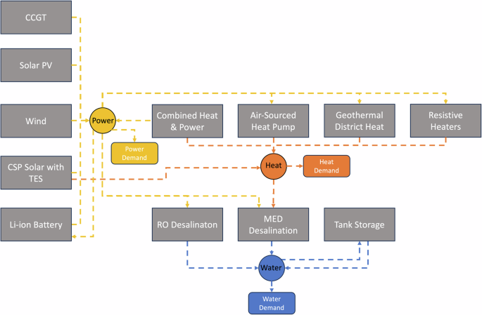
Most technologies produce a specific commodity-heat, power, or water. CSP and CHP produce both heat and power.

Full size image

The optimization determines the investment strategy for five power-generation technologies: combined-cycle gas turbines (CCGT), photovoltaics (PV), concentrated solar power (CSP) with thermal energy storage (TES), onshore wind turbines, combined heat and power (CHP), and batteries. The water sector considers reverse osmosis desalination (RO), multi-effect distillation (MED), and water storage tanks. Heat sector technologies include resistive heaters, air-sourced heat pumps (ASHP), geothermal district heating, CHP, and CSP.

The overall system considers exogenous power, water, and heat demands and endogenous power and heat demand. The breakdown of endogenous power demand includes the four heat generation technologies, the two desalination technologies, RO and MED, while the endogenous heat demand includes only the MED. In this way, the selection of RO and/or MED impacts the size of the power and heat sectors.

The model incorporates the cost and technical parameters of the various technologies (see Supplementary Note 1 for further detail), as well as the renewable resource availability and demand that must be met.

By considering the three sectors simultaneously, the optimization leverages a) the connections between systems, b) the options to invest in alternative storage technologies, and c) the trade-offs between increasing investment costs on capacities and reducing operational costs across the sectors. Decisions for all three sectors are based on cost metrics, renewable resource availability, technology operational constraints, and demand profiles. For example, the link between the power and water systems allows the water desalination capacity to be optimized to increase freshwater production during periods with available renewable energy and reduce production if the batteries are discharging. This operation usually requires additional water desalination and water tank capacities compared with optimal capacities to just supply water demand. If water demand is high and MED and RO desalination facilities are required to desalinate water, the heating and power-generating capacity will be larger to accommodate the water sector.

Low-cost, high-resource technologies will be built first, compared to more expensive technologies with similar resources. In the heat sector, if adding an additional gigawatt of power generation for heating purposes is too expensive, the model may opt to build geothermal or air-source heat pumps, which consume less electricity.

As part of the framework, we expand the optimization model to consider extreme weather days and an assessment of the approximations introduced using representative days. The framework allows the iterative identification of extremes dependent on power-water-heat system designs. It assesses the operational feasibility of those designs over the full weather data (as explained in the Methods section).

Incorporating extremes into planning models results in larger capacity investments and enhances system reliability. Investments in fossil-based generation reduce total costs and improve system reliability compared to a fully renewable system in the face of extreme weather. Fully renewable systems with concentrated solar power and thermal energy storage are less expensive than systems without such investments; however, they are also less resilient to extreme weather conditions. Investment in geothermal heating enables total cost savings but does not impact system reliability.

We apply the proposed energy-sector model to Neom, Saudi Arabia, depicted in Fig. 2. Neom is a futuristic development project in northwestern Saudi Arabia, bounded by the Red Sea, the Gulf of Aqaba, and the vicinity of the border with Jordan. Neom spans 26,500 km² and is expected to operate on fully renewable energy. Because Neom is an area of major infrastructural development, we adopt a greenfield approach and assume annual population and energy demand growth. We assume low, medium, and high future load scenarios with probabilities of 0.3, 0.5, and 0.2, respectively, for all sectors.

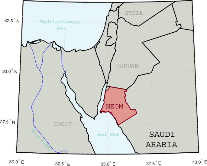
Neom is located in the Northeast region of Saudi Arabia, along the Red Sea.

Full size image

The investment and operating cost data for power sector technologies were obtained from the NREL’s 2022 Annual Technology Baseline³³. The cost data for water desalination and storage technologies were obtained from ref. ³⁴; costs for heat sector technologies were obtained from ref. ³⁵ except for geothermal heating, which was obtained from ref. ³⁶. The costs for the technologies considered are summarized in Supplementary Note 1.

We use a comprehensive weather dataset for the Neom region, which includes direct normal irradiance (DNI), global horizontal irradiance (GHI), wind speed, and temperature data. The dataset covers a period from January 2008 to December 2018, with a spatial resolution of five kilometers. Wind and solar resource data were obtained from refs. ^37,38, respectively, with weather profiles for the Arabian Peninsula generated using reanalysis data from the Weather Research and Forecasting (WRF) model. The model simulations were validated against in-situ observations collected across the region using statistical measures such as correlation coefficient, index of agreement, and normalized mean absolute error.

A conceptual small-scale model of a horizontal, homogeneous geothermal reservoir was set up for a techno-economic analysis of a geothermal system in our multi-sector energy system, as outlined in ref. ³⁶. The subsurface parameters are based on the reservoir conditions of a hydrothermal formation (Al Wajh) representative of the Neom subsurface, which is suitable for geothermal energy extraction. The model is scalable for actual reservoir sizes, energy potential, and energy-extraction schemes. A doublet well pattern, consisting of a vertical injection well and a vertical production well, was assumed, targeting a representative reservoir depth of 2500 m, with an initial reservoir temperature and pressure of 105 °C and 25 MPa. The thermal energy recovered at the surface was assumed to be utilized directly for heating purposes with a utilization factor of 0.85.

The input data, covering costs and technical specifications of all technologies, can be found in ref. ³⁹.

Clustering results: representative regions and days

The Neom region was divided into nine nodes using k-means clustering of the renewable resource data. The spatial partitioning of the region is depicted in Supplementary Fig. 1. Power, water, and heat demand are found across nodes 5, 6, 7, and 9, delineating the central residential/industrial regions of Neom: the Line and Oxagon, respectively⁴⁰. Power-generation and storage facilities can be installed in any of the nine nodes. Only nodes 7 and 9, located along the coast, were selected as candidates for water desalination. Heat sector technologies can only be built in nodes where demand exists or can potentially exist (in case MED is installed). Figure 3 illustrates the complete data set for all weather and demand attributes (in grey), depicting 20 representative days (in black) determined by the k-means clustering. In red are the four extreme days chosen for the fully renewable case. The extreme days have lower cumulative solar irradiance or low wind speeds than the 20 representative days.

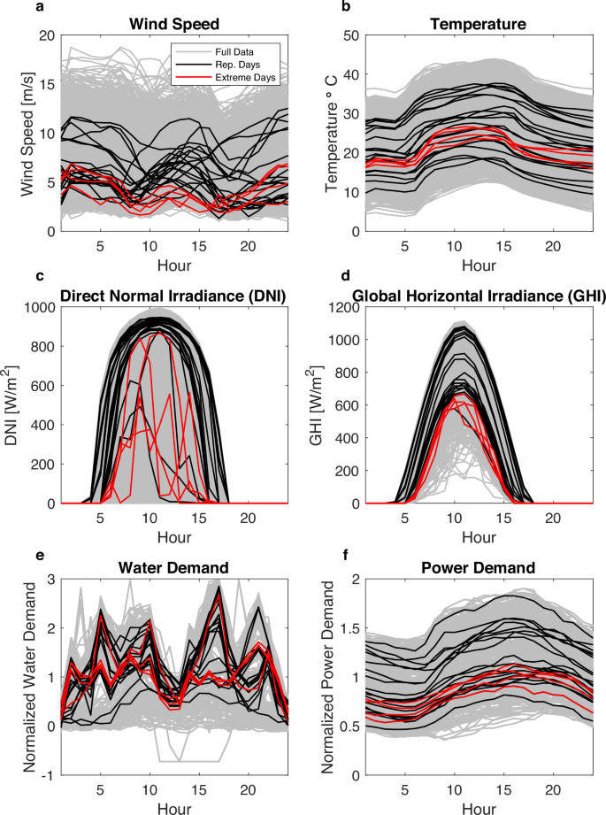
Eleven years of data (in gray) for Neom were clustered into 20 representative days (in black). The attributes used in the clustering are (a) wind speed (in meters per second), (b) temperature (in degrees Celsius), (c) direct normal irradiance (DNI, in watts per square meter), (d) global horizontal irradiance (GHI, in watts per square meter), (e) normalized water demand, and (f) normalized power demand. Data are presented for Region 7. Four extreme days (in red) are depicted from the fully renewable case.

Full size image

Fully renewable system

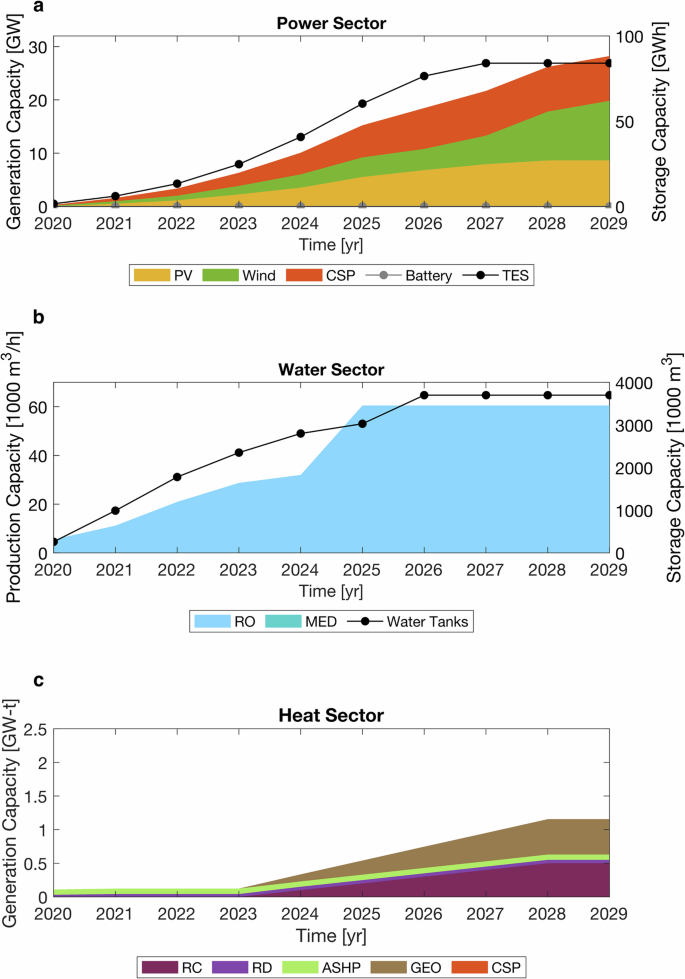
In the case of a fully renewable system, the first iteration—optimization with only the representative days—results in a total generating capacity of 22 GW with a mix of ~40% CSP and 60% wind and PV (equal shares) by the year 2029 as shown in Fig. 4. There are no battery investments; rather, 88 GWh of TES is used as part of the CSP capacity. The water sector comprises 56,200 m³/h of RO capacity and 1.26 million m³ of water tank storage. The heat sector requires 1.6 GW_t of generating capacity with a mix of 32% geothermal, 33% resistive heaters, 5% air-sourced heat pumps, and 30% CSP.

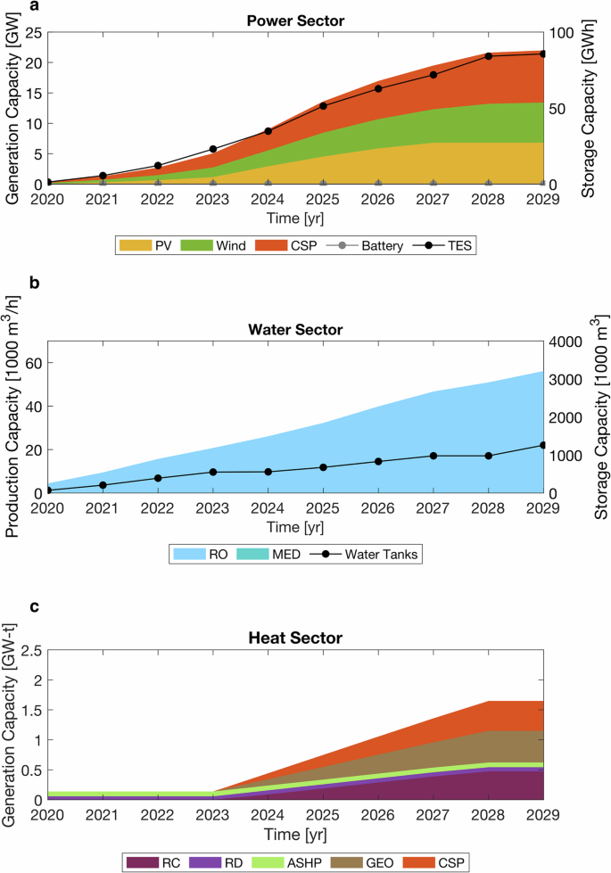
a Power sector generation and storage capacity. Technologies include photovoltaics (PV), wind turbines, concentrated solar power (CSP), batteries, and thermal energy storage (TES). b Water sector production and storage capacity. Technologies include reverse osmosis (RO), multi-effect distillation (MED), and water storage tanks. c Heat sector generation capacity. Technologies include centralized resistant heaters (RC), decentralized resistant heaters (RD), air-source heat pumps (ASHP), geothermal energy (GEO), and concentrated solar power (CSP).

Full size image

We simulated the system operations using the full weather and demand data and the capacities we obtained in the design optimization. The simulation revealed that the system configuration required purchasing large amounts of electricity from the Kingdom of Saudi Arabia (KSA) grid to meet power demand. Figure 5 depicts the final year of the simulation for the high-demand scenario. The power sector struggles to meet electricity demand during the winter season. Meeting the power demand in December is especially difficult due to a marked decrease in solar irradiance and wind speed, as depicted by the weather conditions of the extreme days selected in Fig. 3.

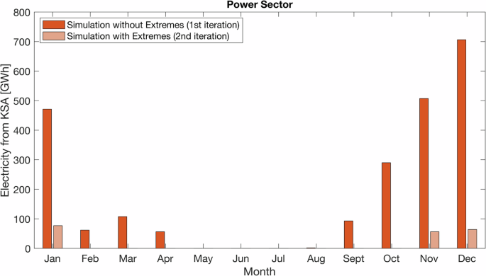
Connections to the KSA grid are more frequent during the winter months compared to the rest of the year. Using extremes reduced the amount of power purchased from Saudi Arabia by 91% for the entire year. (Year 10, High Demand Scenario).

Full size image

Conversely, the system can meet water demand more readily than power demand. The water sector purchases small quantities from KSA during summer and early fall, specifically between June and October. The largest water purchase was in August for 2250 m³, equivalent to 9 GWh of energy consumption. The water purchases for the last year of the time horizon can be found in Supplementary Fig. 2.

Supplementary Fig. 3 shows the operations of three sectors in December for the year 2029. The power sector consistently acquires electricity from the KSA grid, with demand predominantly met by the KSA grid in the evenings.

The addition of extremes results in a 28% increase (up to 28 GW) in total power-generating capacity compared to the first iteration investments. CSP and TES capacity remain the same. However, wind and PV capacities increase by 68% and 28%, respectively (Fig. 6). RO desalination capacity increases by 8% by the end of the planning horizon. Water storage capacity nearly triples in size, suggesting the system requires added flexibility to produce and store more water during specific periods of the year (Fig. 6) compared to the system in Fig. 4. In the heat sector, CSP is no longer used for heating purposes. The total generating capacity decreases by 29% to 1.2 GW_t.

Compared to capacities presented in Fig. 4, power sector capacity increased by 28% compared to the no extremes case. Water tank capacity triples in size. a Power sector generation and storage capacity. Technologies include photovoltaics (PV), wind turbines, concentrated solar power (CSP), batteries, and thermal energy storage (TES). b Water sector production and storage capacity. Technologies include reverse osmosis (RO), multi-effect distillation (MED), and water storage tanks. c Heat sector generation capacity. Technologies include centralized resistant heaters (RC), decentralized resistant heaters (RD), air-source heat pumps (ASHP), geothermal energy (GEO), and concentrated solar power (CSP).

Full size image

In the first iteration, wind turbines are expected to be installed at node 4. However, wind capacity is expanded to nodes 6 and 9 if extremes are considered. Electricity purchases from the KSA grid decrease from 2295 GWh if extremes are not considered to 197 GWh if extremes are considered, a 91% decrease. Fig. 5 shows that electricity purchases occur only in January, November, and December. December still requires electricity from KSA; however, the energy purchased decreased from 706 GWh to 64 GWh.

The system operations for December are shown in Supplementary Fig. 4. Compared to the operations in Supplementary Fig. 3 that do not consider extremes, when extremes are considered, the power sector purchases less power from the KSA grid due to the increased power supply from wind turbines. However, the amount of power spilled increases. Furthermore, the heating sector shifted its generation mix from using CSP to meet nearly 40% of demand to using more resistive heaters when considering extremes.

The cost of having a more resilient energy system—meaning it can better handle extremes—can be quantified as a 13% increase in total costs, as shown in Fig. 7. Individually, the power sector increases by 12%, and the water cost increases by 37%. The heat sector is largely unaffected.

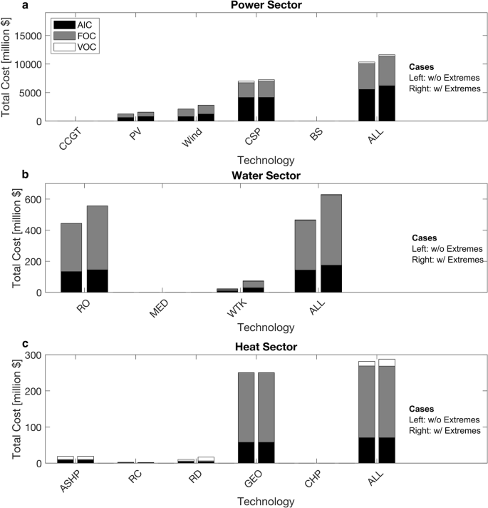
For a fully renewable system, considering extremes increases total costs for the power, water, and heat sectors. The total cost components are broken down into annualized investment cost (AIC), fixed operating Cost (FOC), and variable operating cost (VOC). a Power sector. Costs are shown for technologies, including combined cycle gas turbines (CCGT), photovoltaics (PV), wind turbines, concentrated solar power (CSP), and battery storage (BS). Total costs across all technologies are labeled as ALL. b Water sector. Costs are shown for technologies including reverse osmosis (RO), multi-effect distillation (MED), and water tanks (WTK). Total costs across all technologies are labeled as ALL. c Heat sector. Costs are shown for technologies, including air-source heat pumps (ASHP), centralized resistant heaters (RC), decentralized resistant heaters (RD), geothermal energy (GEO), and combined heat and power (CHP). Total costs across all technologies are labeled as ALL.

Full size image

High penetration renewable system with fossil fuels

Transitioning to a fully renewable system can be cost-intensive¹⁸. Therefore, we explore the cost implications and system reliability of allowing at most 10% of fossil-based generation—CHP and CCGT. The system configuration in the first iteration (without extremes) consists of 29.7 GW of generating capacity–‒44% wind, 37% PV, and 19% fossil fuels, as depicted in Supplementary Fig. 5.

Despite the availability of cost-effective fossil generators, the minimum renewable requirement for annual renewable power generation motivates battery storage capacity to meet demand. However, the energy storage requirements are considerably lower—15 GWh (Supplementary Fig. 5)—compared to previous cases that required over 80 GWh of energy storage (Figs. 4 and 6).

The desalination capacity is exclusively made up of RO desalination. Notably, no investments are made in MED despite the possibility of investing in low-cost heat-generating CHP. The absence of MED investment indicates that heat production cheaper than RO desalination is required by the model.

For instance, MED requires 51 kWh_t of heat to desalinate one cubic meter of water³⁴. If we were to replace the existing RO capacity with MED, the Neom system would require an additional 3.5 GW_t of heating capacity, which would result in a 6% increase in the cost of the system (about 2.6 times the cost for the heat sector).

In the heat sector, introducing fossil-based power allows for a substantial increase in heating capacity, particularly from CHP. By 2029, the heating capacity reaches 2.2 GW_t, a 32% and 88% increase over previous cases. The large rise in capacity highlights the broader impact of incorporating fossil-based power into the system and emphasizes the nuanced interactions between the various sectoral decisions.

Simulating the system operations for ten years with the investment decisions obtained in the first iteration design optimization revealed that the system can meet power demand more reliably than in the fully renewable cases. Supplementary Fig. 6 shows the power purchased from the KSA grid in the last year of the planning horizon. The total energy purchased for the year was 4.44 GWh, with the largest purchases from the KSA grid in July, reaching 2.1 GWh. Compared to previous fully renewable cases with and without extremes, allowing at most 10% renewable power generation decreased annual power purchases by 99.9% and 97.8%, respectively.

Supplementary Fig. 7 depicts the system operations during July. Fossil-based generators are dispatched during some evening hours when solar resources are unavailable, and wind resources are limited.

Water and heat demands are both met exclusively with the capacity in Neom.

Role of CSP for power and heat generation

To study the impact of not using CSP, we turn off the CSP option from the model and run the integrated clustering-optimization method to obtain a system configuration without CSP. After adding extreme days to the set of representative days, a fully renewable system without CSP comprises 40.7 GW of power generation capacity—61% PV and 39% wind as shown in Supplementary Fig. 8. Battery storage capacity is as large as 114 GWh. By comparison, a system with CSP (presented in Fig. 6) has 31% less total power-generating capacity and does not include any battery storage. Instead, it utilizes 84 GWh of thermal energy storage.

With CSP, the water sector builds desalination facilities earlier, reaching its peak capacity by 2025 rather than 2028. Water storage capacity for a fully renewable system with CSP is 45% larger by the end of the considered planning horizon than for a system without CSP.

From a financial perspective, CSP is more cost-effective than PV or wind energy if paired with battery storage. The cost of batteries, which are required to offset the intermittent nature of PV and wind power, increases the total investment needed for these technologies. The cost difference between systems with and without CSP systems is shown in Supplementary Fig. 9. Specifically, investments in CSP result in a 31% decrease in total system costs.

Despite the cost reduction obtained if CSP is allowed, CSP offers less reliability. If extremes are considered, a system with CSP purchased 197 GWh of electricity from the KSA grid; however, a system without CSP purchased 116 GWh—a 41% decrease. Compared to simulation results ignoring extremes, the difference in electricity purchases is larger when CSP investments are allowed. With CSP, electricity purchases totaled 2295 GWh. However, without CSP, the purchased amount decreased to 357 GWh—an 84% decrease, see Supplementary Fig. 10. Water purchases for a fully renewable system without CSP are in Supplementary Fig. 11.

The decreased reliability is due to the presence of thermal energy storage in the CSP technology, which discourages investments in battery storage. TES storage is less flexible as it only stores solar energy, unlike batteries that can store energy from any source.

Role of geothermal for heat generation

Geothermal technologies enable a baseline supply of heat, which can be utilized directly to meet heat demand. Here, we assess the impact of incorporating geothermal district heating. The decision to invest in geothermal heating greatly influences the configuration of the heat sector. Supplementary Fig. 12 and Fig. 6 illustrate the capacity investments for a fully renewable system before and after the integration of geothermal heating, respectively. Integrating geothermal heating effectively displaces resistive heaters while maintaining the overall heat sector capacity.

There is a shift in the water sector, with a 3% and 6% decrease in desalination and water storage capacity, respectively when investments are made in geothermal.

The power sector experiences more pronounced effects from geothermal investments. The total power-generating capacity for a fully renewable system without geothermal is 31 GW, with a generation mix of approximately 29% CSP, 31% PV, and 40% wind. With investments in geothermal heating, the ratio of the generation technologies remains the same. However, the total power-generating capacity decreases by 9% compared to the case without geothermal. The decreased power capacity may be partly attributed to the switch from resistive heaters to geothermal heating.

In the heat sector, the heating capacity for a system without geothermal is 2.1 GW_t with nearly half the heating capacity being CSP. However, with investment in geothermal, total heat capacity decreases by 45% as CSP is no longer used for heating. The resistive heating capacity is nearly half the size.

Resistive heaters typically consume between 1.01 to 1.11 kWh of electricity to produce 1 kWh_t of heat. On the other hand, geothermal systems require less electricity—0.056 kWh, mainly used to power pumps to inject water into the subsurface—to generate 1 kWh_t of heat. The decreased power demand results in cost savings within the power sector, rendering geothermal heating an economically viable option despite its high upfront investment cost. By investing in geothermal heating, total system costs experience a 5.3% reduction.

A more detailed breakdown of the annualized investment, fixed operating, and variable operating costs for the fully renewable case with and without geothermal heating is provided in Supplementary Fig. 13.

Results summary

Tables 1 and 2 show results across technologies and extremes for the high-demand scenario. We present the total commodity purchased from the simulation in Table 1 and the capacities per technology and total system costs from the design optimization in Table 2. The cases presented demonstrate that accounting for extreme days increases system reliability, albeit at a higher total system cost due to the added capacity. The results for the 90% renewable energy case show that the total system cost can be reduced by adding fossil-based generation while keeping the system reliable in the presence of extreme weather days. The use of CSP reduced total system costs and resulted in a less reliable system even when extremes were considered. Supplementary Table 8 summarizes the results for the scenario-weighted average energy, water, and heat purchases.

This study applied an integrated clustering-optimization framework to identify the optimal energy mix for a multi-sector system, factoring in extreme days, various renewable technologies, and even limited fossil fuel generation. The case study was applied to Neom, Saudi Arabia, a region with abundant renewable energy potential and an ambitious goal of operating using 100% renewable power.

Neglecting extremes underestimates the capacity requirements for a fully renewable system, leading to heavy reliance on an external grid, especially during periods with reduced wind and solar resources. Optimizing with extremes leads to strategic geographic placements, notably with wind power, and increased capacity investments to ensure a reliable power supply during these challenging periods. The addition of extremes decreases the total power obtained externally by 91% in a fully renewable system.

The provision to include up to 10% of power from fossil fuels added flexibility and reliability to the energy system. Even a small allowance of fossil fuels greatly mitigated the need for power storage and reduced the demands on renewable energy components, especially during challenging periods. Without considering extremes, a system with at most 10% fossil generation purchased 99% less power from the grid compared to a fully renewable case without extremes. The system also outperformed a fully renewable system that considered extreme days.

CSP emerged as an attractive technology in the renewable mix to decrease the total cost of a fully renewable system. However, the integration of CSP hinders investments in batteries, which are more flexible than the TES used in a CSP system. Because TES can only store thermal energy derived from solar resources, it cannot utilize excess wind resources to help with extreme weather events. When extremes were considered, a system without CSP purchased less power from the KSA grid compared to a system with CSP.

Geothermal energy for heat generation provided another dimension to the optimization, underlining its efficiency compared to resistive heaters. Its integration led to sizable power sector capacity reductions, highlighting the beneficial effects across sectors. Geothermal heating emerges as a long-term economically viable option, driving system-wide cost savings.

Pursuing an optimal renewable energy system for Neom illuminates the importance of comprehensive multi-system modeling. This includes considering extreme days and the synergistic interplay of diverse renewable technologies. As the world navigates the nuances of transitioning to cleaner energy sources, insights from such studies are important in steering policy, investment, and infrastructure decisions to create resilient, sustainable, and economically viable energy landscapes.

The optimization problem is formulated as a two-stage stochastic program⁴¹ with scenarios capturing the uncertain demand for the three sectors, a planning period of ten years, and an hourly resolution. Each scenario corresponds to a combination of uncertain power, water, and heat demands, which depend on future population projections. The first-stage variables are annual investment decisions on generation and storage technologies, while the second-stage variables are operational decisions based on the realization of the uncertain demand⁴². The objective function minimizes the total cost, which includes annualized capital, fixed operating, and expected variable operating (dependent on the scenario, ω) costs. The objective function is subject to investment and operational constraints for all sector technologies. Investment constraints define a range of annual investments and cumulative capacity. The operational constraints define the production and storage values of all technologies. A compact formulation is given by:

where CAPEX_f, FOM_f, and VOM_ω,f,o,t depend on the capacities and operational variables occurring in the constraints. Supplementary Notes 2 provides a detailed problem formulation and nomenclature list. In essence, CAPEX_f is the capital expenditures in year f of adding new capacity for all the technologies, and FOM_f is the fixed operating cost incurred in year f, dependent on the existing capacities. The VOM_f is the total variable operating cost of the system in year f, considering generation and storage costs based on the operational decisions. The variable cost is incurred every hour, t, for each representative day o. α_ω and β_o are fixed parameters that correspond to the probability of scenario ω and the weight (number of days of the year) of the representative day, o, respectively. This formulation uses representative days to approximate the renewable resources and demand over a year. Renewable potentials and demands are modeled at representative regions

While transmission constraints are relevant in long-term planning expansion problems for power and water, we do not consider them for either sector to reduce model complexity. We assume that transmission will be built to accommodate the predicted maximum capacity. Heat demand is met at a nodal level but does not allow trade between nodes because heat cannot be transported long distances due to losses. Transmission constraints for the heat sector are, therefore, not relevant.

The uncertainty associated with the technologies’ prices is not considered and represents a limitation of the present implementation because variations in future production costs may lead to different investment strategies. The latter would need to be assessed through an extended model that simultaneously accounts for the availability of energy resources, complementarity, and match of supply and demand.

Our optimization model assumes a greenfield approach motivated by the specific case study we consider. However, it is also relevant for cases in which a renewable-based system is required to meet the target energy demand of a city, community, region, or industrial complex. For fully renewable cases, the model formulation is a linear program; for cases with fossil-based power generation, the model is a mixed integer linear program due to the introduction of binary variables.

Weather resources and spatio-temporal representation

Modeling the decisions for a capacity planning model deals with vast amounts of data, often spanning hourly (or even finer) temporal resolutions over several years. These decisions also span multiple locations as it is necessary to determine where and how much to build within a specified region. A well-known approach to compress weather and demand data is to replace yearly periods with hourly resolutions with representative days to reduce the computational burden. This approach involves selecting a subset of days that capture the typical behaviors and variations of the system throughout the region and a given period. Therefore, instead of optimizing the operations of a system for every hour of the year and fine-scale location, one uses a smaller set of representative regions and days.

Representative regions enable the aggregation of high spatial resolution weather data that captures weather patterns across different regions and weather attributes. An alternative approach is to use existing regions, often based on political boundaries, and use the average or median of the various weather attributes to represent said region. In our study, we apply k-means clustering to delineate nodes with similar weather conditions.

We applied k-means clustering to group 11 years of weather data and a normalized demand data set into representative days (spanning 24 h). Given the high variability of renewables, representative days were chosen. Using 24-hour days allows one to capture the diurnal variation of solar and wind resources. With several representative days, historical variations throughout the year are ascertained.

The days were clustered based on the water and power demand, wind and solar availability, and temperature. The number of clusters can be selected using a trial-and-error scheme, in which the expansion planning optimization is solved recursively over an increasing number of days until the decision variables stabilize.

By optimizing the performance of the overall system over representative days, the optimization can capture much of the variance observed throughout the year. However, there are limitations to using representative days:

1. 1.

   The most relevant limitation concerns missing extreme weather conditions. While representative days capture variance, the days selected are averages or near averages, which smooth out extreme conditions. This effect is discussed, for example, in ref. ²⁸. The selected days often miss extreme events critical for system reliability, such as prolonged heat waves or unusual renewable generation caused by atypical weather patterns. As a result, the decisions made based on the optimization might be infeasible if these rare but important events occur and, therefore, underestimate the system’s total cost.

2. 2.

   Representative days are inadequate for systems with long-term energy storage, such as hydro reservoirs, with cycles longer than one day, as discussed in ref. ²³. In this work, the batteries and the thermal energy storage tanks have much smaller cycles than hydro reservoirs. However, their cycle can still be longer than one day, depending on the renewable resources available and power demand.

Therefore, a solution method to minimize the impact of these limitations on the planning of power-water-heat systems is warranted.

Solution method incorporating extreme days

We propose an integrated clustering-optimization method that considers extreme weather days and an assessment of the approximations introduced by using representative days. The overall goal is to plan a reliable power-water-heat system.

The definition of extreme weather days is an intricately complex task tied to the specific configuration of the power system. For instance, a system heavily reliant on solar power would consider prolonged cloudy days extreme. Conversely, days with little to no wind might be extreme in a system mainly powered by wind turbines. One potential approach to capture these extreme days is to increase the number of representative days used. However, if the extreme days are large outliers in the dataset, such an approach may require too many additional days to capture those extremes, rendering the model intractable.

The proposed method iteratively identifies extremes dependent on power-water-heat system designs and assesses the operational feasibility of those designs over the full weather data. Our method is based on the following steps:

1. i.

   use k-means clustering to identify representative days from a full weather and demand dataset;

2. ii.

   solve the design optimization problem (1) over the representative days identified in i);

3. iii.

   fix the generation and storage capacities obtained in ii) in problem (1) and run a simulation on the operations over the full weather data;

4. iv.

   assess if the system meets the external supply tolerance;

5. v.

   identify extreme weather and demand events based on the solution of the problem described in iii);

6. vi.

   add the extreme events to the set of representative days; and

7. vii.

   iterate the process by re-solving the design optimization problem in ii).

This approach is inspired by the methodology proposed in³¹, which we adapted to a fully renewable energy system coupling multiple sectors–water, power, and heat–and to a near fully renewable one. Figure 8 summarizes the iterative workflow of our approach.

The representative days are identified in the first iteration using the k-means algorithm. During the clustering, the index of the days in the dataset is tracked, and consequently, the selected days are ordered chronologically. It is important to note that numerous other data reduction methods, such as those explored in ref. ²⁰, can be used to select representative days. The solution to the problem (1) provides the optimal system configuration given the representative days selected. From this configuration, the capacities to build are fixed in the operations simulation, which is solved over the full weather and demand data. At this stage, the water, energy, and heat balances are modified to accommodate slack (nonnegative) variables that represent the additional water, energy, or heat required from external sources if the system is operated over the full weather and demand data instead of the representative days. These slack variables are represented by ({s}_{omega ,n,f,o,t}^{{{{rm{pwr}}}}},{s}_{omega ,n,f,o,t}^{{{{rm{wtr}}}}}) and ({s}_{omega ,n,f,o,t}^{{{{rm{heat}}}}}) in the following balances (These are compact versions of the balances presented in the Supplementary Note 2.),

• energy balance:

  $${sum}_{n}left({g}_{omega ,n,f,o,t}^{{{{rm{pwr}}}}}+{b}_{omega ,n,f,o,t}^{{{{rm{pwr}}}},{{{rm{out}}}}}+{s}_{omega ,n,f,o,t}^{{{{rm{pwr}}}}}right)={sum}_{n}left({D}_{omega ,n,f,o,t}^{{{{rm{pwr}}}}}+{b}_{omega ,n,f,o,t}^{{{{rm{pwr}}}},{{{rm{in}}}}}right),quad forall omega ,f,o,t$$

  (2)

  where ({g}_{omega ,n,f,o,t}^{{{{rm{pwr}}}}}) represents the total electricity production by all technologies selected, ({b}_{omega ,n,f,o,t}^{{{{rm{pwr}}}},{{{rm{out}}}}}) and ({b}_{omega ,n,f,o,t}^{{{{rm{pwr}}}},{{{rm{in}}}}}) represents the total batteries inputs and outputs, ({D}_{omega ,n,f,o,t}^{{{{rm{pwr}}}}}) represents the electricity demand, and ({s}_{omega ,n,f,o,t}^{{{{rm{pwr}}}}}) is the slack variable used to account for the external electricity needed;

• water balance:

  $${sum}_{n}left({p}_{omega ,n,f,o,t}^{{{{rm{wtr}}}}}+{t}_{omega ,n,f,o,t}^{{{{rm{wtr}}}},{{{rm{out}}}}}+{s}_{omega ,n,f,o,t}^{{{{rm{wtr}}}}}right)={sum}_{n}left({D}_{omega ,n,f,o,t}^{{{{rm{wtr}}}}}+{t}_{omega ,n,f,o,t}^{{{{rm{wtr}}}},{{{rm{in}}}}}right),quad forall omega ,f,o,t$$

  (3)

  where ({p}_{omega ,n,f,o,t}^{{{{rm{wtr}}}}}) is the freshwater production, ({t}_{omega ,n,f,o,t}^{{{{rm{wtr}}}},{{{rm{out}}}}}) and ({t}_{omega ,n,f,o,t}^{{{{rm{wtr}}}},{{{rm{in}}}}}) are the inputs and outputs of the water storage tanks, ({D}_{omega ,n,f,o,t}^{{{{rm{wtr}}}}}) is the freshwater demand, and ({s}_{omega ,n,f,o,t}^{{{{rm{wtr}}}}}) is the slack variable used to account for the external water needed; and

• heat balance:

  $${g}_{omega ,n,f,o,t}^{{{{rm{heat}}}}}+{s}_{omega ,n,f,o,t}^{{{{rm{heat}}}}}={D}_{omega ,n,f,o,t}^{{{{rm{heat}}}}},quad forall omega ,f,o,t$$

  (4)

  where ({g}_{omega ,n,f,o,t}^{{{{rm{heat}}}}}) is the heat production, ({D}_{omega ,n,f,o,t}^{{{{rm{heat}}}}}) is the heat demand, and ({s}_{omega ,n,f,o,t}^{{{{rm{heat}}}}}) is the slack variable used to account for the external heat needed.

In the operations simulations, positive values of slack variables are used to identify periods during which the generation and storage capacities installed are insufficient to meet the demand due to the consideration of the full scope weather and demand data. Days with positive slack value for a commodity at any hour are labeled as infeasible. Of the infeasible days, the days with the largest cumulative slack values are classified as extreme days. An extreme day or a series of extreme days (with the largest slack values) can be added to the set of representative days with the weights of the extreme days calculated by

where N^infeas,days, is the number of infeasible days, ({N}^{{{{rm{extr}}}},{{{rm{days}}}}}) is the number of extremes that will be added to the set of representative days, ({{{mathcal{O}}}}) (({{{{mathcal{O}}}}}^{{{{rm{extr}}}}}) is a subset of ({{{mathcal{O}}}}) containing the extreme days), and ({N}^{{{{rm{sim}}}},{{{rm{days}}}}}) is the number of days that are in the simulation horizon.

For a system with multiple sectors, each commodity balance constraint will have a slack variable with multiple sectors having a nonnegative slack value. Therefore, when selecting the extreme days, the modeler must assess from which sector to select the extreme days. Possible options include 1) selecting the extremes from the sector with the largest slack values relative to the demand, 2) selecting a day (or days) with the largest slack value from each sector, and 3) selecting the extremes from the sector that is most constrained. If the maximum value slack (for the chosen sector) over the scenarios is below a specified tolerance, then the system configuration obtained from problem (1) can handle the extreme scenarios, and the iterative process represented in Fig. 8 stops. Otherwise, the solution of the design optimization problem (1) is repeated with the set of representative days plus the extreme days identified. The process is repeated until the slack variables are below a specified tolerance.

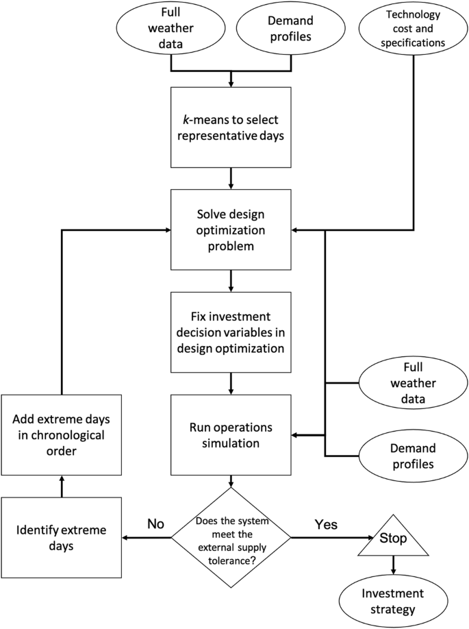
The workflow involves identifying representative days via k-means clustering on an 11-year data set of weather and demand profiles. A design optimization is performed over the representative days to identify a design strategy. An operations simulation is run with fixed design variables over the full weather and demand data. Extreme weather and demand events are identified based on the solution of the simulation. Extreme days are added to the representative days, and the design problem is resolved.

Full size image

Remarks

1. i.

   Besides k-means, several other clustering algorithms, such as Gaussian mixture models, are available⁴³ and can be used to reduce the problem size. The present methodology may be adapted to these alternative approaches.

2. ii.

   The extreme days are drawn from the full weather data. Adding them to the design optimization aims towards planning a more robust power-water-heat system for conditions not captured initially by the representative days.

3. iii.

   If multiple extreme days are included in the design optimization, the sequence of extreme days may enforce worse conditions than those resulting from the extreme days distributed through the years in the full weather data. This approach can, in turn, lead to overestimating the capacity and, therefore, suboptimal solutions.

4. iv.

   At each iteration, the design optimization is solved without fixing previous design variables, which enables the design optimization to adapt to the inclusion of extreme weather days.

5. v.

   One or more extreme days can be added to the design optimization at each iteration. The number of extreme days to add is a parameter of the method that influences the number of iterations and can be tuned to the specific input data for the optimization problem.

6. vi.

   The external supply tolerance indicated in step iv) of the method to incorporate extreme days and in Fig. 8 can be used by the decision-maker as an external budget of energy to prevent high investment costs on 100% renewable systems that cover supply over extreme days. On the other hand, setting the external supply tolerance to zero enables the quantification of the storage and generation capacities, costs, and external energy increments at each iteration. This information can support the decision-maker on alternative strategies to handle the extreme days, such as contracts with neighbor power systems or investing in demand-side management strategies.