The study presented in this paper creates a unique and robust dataset for Sustainable Household Energy and Environment Resources Management (SHEERM). This dataset encapsulates cross-sectional data of household electrical load, energy cost, and on-premises solar energy production, directly linked to solar irradiation and weather parameters, all in the context of thirteen real-world household scenarios over nearly three years with no sub-metering. It is a significant step forward in line with the strategies proposed by previous research, enhancing our understanding and enabling effective optimization of energy utilization. Previous studies, represented in Table 1, have examined individual aspects of household energy consumption and solar energy, focusing either on solar energy production or consumption, with limited integration of different components such as energy, weather conditions, battery capacity, or energy price.

Among the available datasets, which include the DKA Solar Centre¹ and NSRDB data², it is essential to note the limitations of these datasets. For instance, the DKA Solar Centre in Alice Springs datasets contains data from several solar panels monitoring energy generation and a few weather features such as temperature, pressure, and wind speed/direction. However, a significant problem occurs as there are numerous instances of missing data, and in most datasets, there’s a lack of documentation regarding the metrics of each variable. This absence of clarity can pose significant challenges during data analysis. On the other hand, the NSRDB data offers a broader range of weather features compared to the DKA Solar Centre.

Most of the data used in the works surveyed is typically not disclosed^{3,4,5,6,7,8,9,10,11,12,13,14,15,16,17} or, if claimed to be disclosed in the paper, is often unavailable upon further investigation^18,19,20,21. Several papers use simulated data for their purposes^22,23,24. This lack of transparency and availability can make comparing results challenging or exploring alternative methodologies using the same datasets.

Our study builds upon these gaps and extends the literature by providing an integrated, comprehensive, and specific dataset that facilitates an interconnected analysis. This study collected, integrated, and standardized data from different sources to create a complete dataset with information about solar energy, weather conditions, household load, and energy grid prices.

Household load consumption data was obtained through smart meters installed in a set of thirteen houses located over different regions of Portugal, representing all of its regions. Related datasets, such as CoSSMiC^25,26 and Ausgrid²⁷, also provide load and solar energy measurements. However, they are related to different regions from SHEERM, which comprises data from Portugal. Furthermore, the SHEERM dataset offers a more comprehensive view of weather conditions, including details, for instance, on temperature and cloud coverage. It also explicitly specifies the solar panels’ characteristics and the solar energy they generate. SHEERM aims to contribute more data for a broader analysis of power consumption and photovoltaic power generation.

The data on grid energy prices was retrieved from the Ember Climate website²⁸, which offers a range of publicly available datasets on climate data and electricity prices.

The dataset for weather conditions was obtained from the National Solar Radiation Database (NSRDB)²⁹, which provides high temporal and spatial resolution data, including the three most widely used measurements of solar irradiation – global horizontal irradiance (GHI), direct normal irradiance (DNI), and diffuse horizontal irradiance (DHI) – along with other meteorological data.

The solar panels have been carefully selected from commercial stores where they are currently available for purchase. These panels are being used by electrical companies to be installed on rooftops, given the region’s specific climate and sunlight conditions. They are designed to capture data on solar energy generation effectively. Additionally, some models come equipped with sensors to monitor weather conditions, providing a comprehensive solution for solar energy management.

Integrating solar production data, weather variables, and residential energy needs in the SHEERM dataset significantly enhances its usability for various analytical purposes. It can foster advancements in renewable energy forecasting, aid in developing climate-sensitive environments, improve grid management practices, and assist in formulating energy-efficient policies. Therefore, the SHEERM dataset holds immense practical value for reuse and potential applications in various domains, including environment, urban planning, users’ cost reduction, and energy saving.

By providing this extensive dataset, our study aims to assist in designing new energy systems that enhance sustainable energy strategies and demonstrate their potential in accelerating the transition towards renewable energy and carbon neutrality. It serves as an important dataset for researchers and policy-makers and is also intuitively designed to benefit a larger community, leading sustainable development towards reducing dependence on fossil fuels.

Renewable energy generation has gained increasing global recognition and importance due to its availability and potential to limit the escalating of environmental concerns and achieve sustainable development. Adopting solar energy in individual houses can have significant implications for accomplishing the Sustainable Development Goals (SDGs) set by the United Nations^30,31.

This study presents a substantial dataset encompassing four key elements of energy production and consumption: household energy needs, weather conditions, solar power generation, and market energy costs. This dataset is valuable for analyzing the complex interplay between these variables, thereby driving energy efficiency, sustainable strategies, and cost-effective planning.

The household energy load data represents the energy demand of a particular house, and understanding it will lead to time-efficient energy management that correlates with the demand schedule and production. Additionally, the weather data encapsulates different environmental parameters such as temperature, sunlight hours, cloud information, etc. Since these aspects directly influence the solar panel efficacy, understanding the weather patterns can help us maximize energy production and extend the panels’ functional life. Analyzing weather data and solar panel performance can offer interesting insights into optimal weather conditions for maximum energy output.

Lastly, comprehending the market energy prices is indispensable to analyzing the cost versus benefit of installing solar energy production systems. This analysis helps manage energy storage systems (batteries), energy production, and peak price timelines to guarantee the most effective strategy.

Together, this multivariable data promises comprehensive insights into household energy production and consumption, aligning with SDG 7 since the dataset can be used to optimize solar energy production and distribution and contribute to universal energy access and sustainability. Moreover, enhanced and efficient utilization of solar energy data can stimulate innovation in energy technologies and facilitate the sustainable transformation of infrastructures (SDG 9). The data is also relevant for improving urban planning and the more effective integration of renewable energy resources to ensure sustainable urban development (SDG 11), and it can help reduce reliance on fossil fuels by facilitating a deeper understanding and efficient usage of solar energy, thus assisting in mitigating climate change (SDG 13).

However, the effective implementation and management of solar energy require a comprehensive understanding and holistic insights into different parameters, including solar energy production, weather conditions, and household load requirements.

Based on the outputs generated by a deep analysis of the SHEERM dataset, governments can establish supportive frameworks to drive innovation, attract investment, and stimulate market growth in the renewable energy sector^32,33. One practical result may be the creation of community solar projects, which allow multiple households or institutions to share the benefits of a single solar installation. This model democratizes access to solar energy, enabling those without suitable rooftops to participate in and benefit from renewable energy generation.

Another outcome of a deep understanding of the data in the SHEERM dataset may be new advancements in battery technology. Dynamic, adjustable, and improved energy storage solutions enable better management of intermittent energy sources. This increases the reliability of renewable energy systems and facilitates their integration into the existing energy grid³⁴. Innovative approaches to vehicle charging technology also contribute to a more sustainable energy landscape. By understanding household behavior, smart systems can maximize the usage of renewable energy sources for vehicle charging³⁵.

Additionally, smart grids can optimize grid energy distribution by integrating household forecasting information, allowing utilities to optimize energy flow and improve demand response capabilities^36,37. Thus, the SHEERM dataset offers significant practical value for reuse and potential applications across various domains.

The data presented in the dataset was acquired through particular methods, carefully designed experiments, and computational processing for straightforward interpretation. Details about the data collection processes are explained further.

Household Energy Consumption Data

One of the main goals in energy-related research is the study of household energy consumption to help users reduce their monetary costs and environmental footprint. Thus, it is crucial to have datasets with household energy consumption information.

For the SHEERM dataset, thirteen distinctive houses in Portugal were equipped with smart electric energy meters (certificate equipment according to the EC Directive 2004/22/EC³⁸), which measure and record household energy consumption every 15 minutes.

Each smart meter applies a simple outlier detection based on a threshold. A high value (10 kWh) was used as the threshold to ensure minimal restriction on data acquisition and to collect possible spikes that may occur in household energy consumption. The sampled value is considered for further sending if it is within the defined threshold. Otherwise, it is dropped, creating missing data. Then, linear interpolation is used to estimate any missing data point, ensuring continuous data in the time series. These devices communicate the measurements remotely to a central server, simplifying data storage and retention. We used a reliable transmission protocol to ensure the data was delivered to the server.

On the server side, we implemented a neural network with two dense layers of 64 neurons each, two relu activation functions, and one dense neuron as the output layer. The neural network was configured to consider a sliding window of 3000 data samples (+/- 1 month). It is used to predict and compare the next data point with the data point received. This network runs every period (every 15 minutes) when a supposed data point arrives. A delay tolerance approach is also applied, allowing a 2-minute delay. The predicted value is compared if the data point is received on that interval. If a deviation exceeding a predefined threshold is detected, the received data point is replaced with the predicted value. If the data point is not received within the 2-minute, a missing value is assumed, and the data series is filled with the predicted value. This approach effectively filters the data by removing outliers while preventing the introduction of missing values^39,40, creating a reliable dataset.

The houses included in this study and their locations are summarized in Table 2. Six of these residences (houses 1, 2, 3, 4, 5, 6) are located in a region with relatively mild seasons, where winter temperatures typically range between 5-10 degrees Celsius and summer temperatures fluctuate between 25-40 degrees Celsius. These houses are noted for their excellent insulation and effective thermal comfort indicators, significantly influencing energy consumption patterns.

Three selected houses (houses 8, 9, 10) are situated in a region well-known for its extreme temperatures in Portugal, offering a contrasting dataset that unveils unique energy consumption perspectives. With winter temperatures known to dive to 0-4 degrees Celsius and summers catching a surge to 35-45 degrees Celsius, these houses provide insights into energy usage. However, these houses are equipped with specialized heating systems that operate without electricity. These systems ensure warmth and comfort while reducing reliance on the electrical grid.

The other houses near the sea benefit from the ocean’s moderating influence. This location ensures a relatively stable and moderate temperature throughout the year, creating a comfortable living environment regardless of the season.

Ultimately, our dataset, consisting of comprehensive historical household energy consumption recorded every 15 minutes for these thirteen houses over the past months and years, offers a panoramic view of usage patterns. It considers the variations of different seasonal temperatures, influencing the thermal comfort indicator and energy consumption. Despite Portugal being a small country, the large temperature amplitudes between the various zones make it a good case study candidate for collecting this type of data.

To enrich our data, and since there is a relationship between energy usage and factors such as the time of day, whether it’s a weekend or not, and the season, several new variables were engineered from the Date and Time variable. These include the “Day of the week�, which indicates the day of the week the data is (e.g., Monday, Tuesday, etc.), the “Daytime� (e.g., daytime or nighttime), and the “Season� (e.g., spring, summer, autumn, winter).

Weather Data

Obtaining a dataset that includes weather and solar irradiation data can be challenging, especially if real data is desired. Weather datasets are more readily available through Application Programming Interfaces (APIs), offering a convenient source of up-to-date information. Some notable APIs include Meteostatt⁴¹, a freely accessible weather and climate database providing temperature, wind speed, and pressure information. However, it lacks data on solar irradiation, and the granularity of the data is limited to the hour. In this case, it would be preferable to have data recorded at intervals of 30 minutes or less for more accurate predictions. Another API worth mentioning is the National Solar Radiation Database (NSRDB)²⁹, which, despite offering similar features to its web-based data extraction counterpart, is not updated regularly in the area covered by this study (i.e., Portugal). Additionally, other APIs, such as the Weather API from API Ninja⁴², or OpenWeatherAPI⁴³ either require a subscription plan or lack the necessary features. Moreover, finding datasets that seamlessly integrate weather and solar irradiation data adds a layer of complexity to this task.

To address these limitations, our dataset includes data from the National Solar Radiation Database (NSRDB) for the specific locations of the houses under consideration. We selected data from 2021 to 2024, using all available features to ensure comprehensive coverage. The information was provided through email by the National Renewable Energy Laboratory and organized into CSV files.

The features in the dataset include Timestamp, Temperature, Clearsky DHI, Clearsky DNI, Clearsky GHI, Cloud Type, Dew Point, DHI, DNI, Fill Flag, GHI, Ozone, Relative Humidity, Surface Albedo, Pressure, Precipitable Water, Wind Direction, Wind Speed, Solar Azimuth Angle (rad) and Solar Zenith Angle (rad). Each row represents a 15-minute interval, with the data corresponding to surface cells measuring 0.038 degrees in both latitude and longitude, equivalent to approximately 4 Ã— 4 km in size²⁹.

From this dataset, several features were derived from existing ones, while others were added. For instance, the NSRDB data originally included information on year, month, day, hour, minutes, and seconds, each in separate columns. To streamline and simplify the data handling process, these six separate columns were consolidated into a single “Timestamp” column, which now contains all temporal information in a unified format. This change enhances data usability and clarity by replacing multiple time-related columns with a single timestamp representation.

Other features that have been added to the dataset include the solar azimuth (rad) and solar zenith angles (rad), both computed using the sun-position-calculator⁴⁴ and considering the position (latitude, longitude) of each house. This enhancement contributes to a more comprehensive dataset, facilitating future predictive modeling related to solar irradiation. Both solar azimuth and zenith angles are influential factors in determining the solar irradiation received at a specific surface, making them valuable additions for accurate solar power generation predictions.

Solar Power Generation Data

Considering the weather data, it is possible to calculate the predicted amount of power P_G a solar photovoltaic (PV) panel could generate according to Eq. (1)^45,46:

wherein η is the conversion efficiency (%) of the solar cell array, S is the array area (m²), t₀ is the outside air temperature (°C), and Δ is the solar irradiation (kW/m²) on the PV panel.

A question that arises is which solar irradiation (Δ) should be employed to calculate the energy generated from a given solar panel. It is common practice to utilize the Global Horizontal Irradiance (GHI) when determining the energy output of solar panels. GHI accounts for both Direct Horizontal Irradiance (DHI) and Direct Normal Irradiance (DNI), making it a comprehensive metric for assessing the total solar irradiation received on a horizontal surface (Fig. 1). In the context of solar energy calculations, GHI provides a holistic view of sunlight, incorporating the direct sunlight that reaches the surface and the diffuse sunlight scattered by the atmosphere. This makes GHI a commonly used parameter for estimating the overall energy potential of a solar panel.

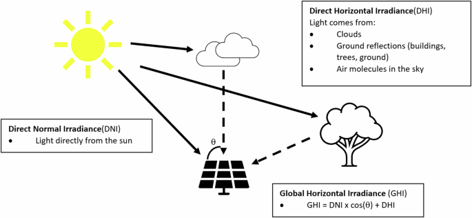
Illustration of the different types of irradiation captured by a solar panel.

Full size image

As defined in⁴⁷, the solar irradiation (Δ) is computed according to Eq. (2):

Note that θ represents the incidence angle of solar irradiation on the panel surface⁴⁸, and it is defined by Eq. (3):

wherein θ_s is the solar zenith angle, γ_s is the solar azimuth angle (i.e., the angle between the north and the sunbeam as projected on the horizontal plane), β is the tilt angle of the PV panel surface to the horizontal, and γ is the PV azimuth angle (i.e., the angle between the north and the normal of the PV panel surface as projected on the horizontal plane).

When applying the analytical expression (Eq. (1)) provided by⁴⁵, it becomes evident that numerous factors, including the measurement of solar irradiance, estimation of PV cell temperatures and the efficiency of the system, influence the forecasted power output of PV generations.

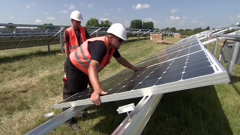
Figure 2 illustrates two solar panel configurations for exemplification.

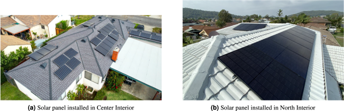
Examples of solar panel installation in Portugal.

Full size image

To predict the amount of photovoltaic energy that can be generated at each location of the selected houses, we conducted a comprehensive search to find specifications for typical solar panels used in households across the Portuguese regions covered by our dataset. Our research identified the models represented in Table 3.

To predict the energy each house could produce with an installed photovoltaic panel, we matched each house in our dataset with a corresponding solar panel presented in Table 3. Table 2 shows this association, each house’s relative location, and the panel’s positioning (tilt angle).

Based on those tables (Tables 2 and 3), we compiled a dataset that represents the amount of energy generated at each location. Equations (1), (2) and (3) were used to compute the data related to solar power generation. The exact location of each house was used for these calculations. However, due to privacy concerns, this information was omitted from Table 2 and replaced by the name of the corresponding region of each house in Portugal.

Market Energy Price Data

Another essential variable in the SHEERM dataset is related to how much a household owner needs to spend on electricity (market electricity price). This information can be beneficial for calculating the electricity usage from the grid given the load of the houses, and it can also be used for prediction or recommendation purposes to save energy and reduce costs. Information regarding the market prices of Portugal was obtained from the Ember-climate website²⁸, and the data consists of European wholesale electricity price data. The file downloaded from the website contains information about gross energy prices in various European countries. The dataset corresponding to Portugal has 76,680 rows and five columns. The features present in the SHEERM dataset are the country information (Country and ISO3 Code), the local date-time and its reference in UTC format (Datetime (Local) and Datetime (UTC)) and the electricity price in EUR/MWh (Price). To simplify the SHEERM dataset, the country information and the variable Datetime (UTC) were removed, maintaining only the DateTime (Local).

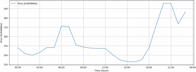
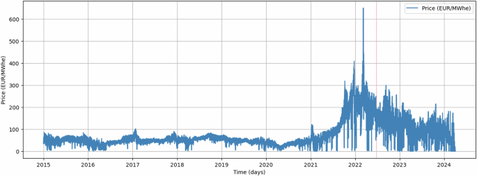
Each row in the dataset corresponds to the price of electricity at every given hour. Considering the limited number of features (restricted to time and cost) available for applying a prediction model information, it becomes apparent that creating a robust model would likely require additional variables. A simple analysis reveals that electricity prices vary according to the time of day (Fig. 3). Additionally, when examining monthly trends (Fig. 4), no clear pattern emerges across the days of the month. However, distinct patterns are evident when considering different months. Lastly, a similar behavior can be identified for the year analysis (Fig. 5). Figures 3, 4, and 5 represent an example of each analysis. However, numerous analyses can be done on our data. The SHEERM dataset comprises data from 2015 until the end of 2024 regarding market energy prices.

Market Energy Price data for a given day (highlighted in pink in Figs. 4 and 5).

Full size image

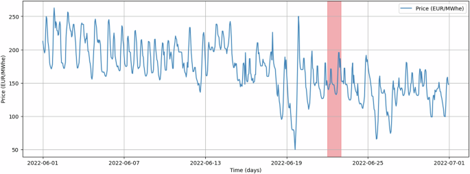
Market Energy Price data for a given month.

Full size image

Market Energy Price data per year in the range of 2015 and 2024.

Full size image

Introducing new features to enhance the model’s predictive capabilities is important. Similar to the Weather Data, to enrich the Market Energy Price Data, we added features such as “Day of the week� (e.g., Monday, Tuesday, etc.), “Daytime� that can assume a value of daytime or nighttime, and “Season� information (spring, summer, autumn or winter). This information makes the dataset more useful for predictive models.

For this work, the SHEERM dataset⁴⁹ is organized into four main parts: one for household consumption data (Load), one for electricity price data (Price), one for weather information (Weather), and one for the photovoltaic generation (PV Generation). The household consumption data (Load) is divided into two parts: raw data and processed data. The raw data corresponds to the data received by the server. It includes some missing data that results from network disconnections and grid-off times. The processed data corresponds to the data stored by the server. As described in the Methods Section, the server implements a machine-learning algorithm to predict and compare the next data point with the data point received. This allows us to identify and remove any outliers and fill gaps originating from missing data. The Household Consumption data (Load), Weather, and PV Generation information are from 13 houses spread across Portugal.

Household Consumption Data (Load)

Data from 13 households was collected across Portugal, generating 13 CSV files, one for each household. Each CSV file contains 3 variables, one of which is the Date, which refers to the day of the reading. In contrast, the second variable has information on the reading time, and the third represents the house power consumption for that specific time in kW.

The SHEERM dataset includes raw and processed data related to household consumption. Table 4 shows the range of dates, the total number of rows, the number of missing rows and their ratio, and the total number of rows after data processing on the server.

Table 4 shows that the dataset covers almost 3 years of data, including, on average, 82358 records per house. Regarding the missing data, the overall ratio of missing data is relatively low, which means that their impact on statistical models and machine learning algorithms is significantly reduced. Additionally, this low ratio means fewer gaps must be filled, allowing for more accurate trend identification and greater confidence in the validity of the dataset. Figure 6 presents a histogram illustrating the distribution of gap lengths. From Fig. 6, we observe sporadic instances of single missing samples, indicating brief interruptions in data transmission. However, gaps of up to 10 consecutive missing samples are present, suggesting few periods of sustained connectivity issues. The most significant data losses are observed in houses situated in areas where the network connection is unreliable. These regions likely experience intermittent signal strength fluctuations or high latencies, contributing to the prolonged data gaps.

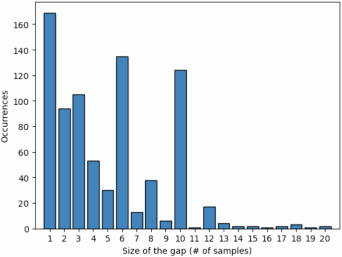
Histogram of gaps’ length.

Full size image

In terms of household consumption data included in the SHEERM dataset, as an example, Fig. 7 shows the consumption values for Houses 1 and 2 for a specific day (2021-05-01).

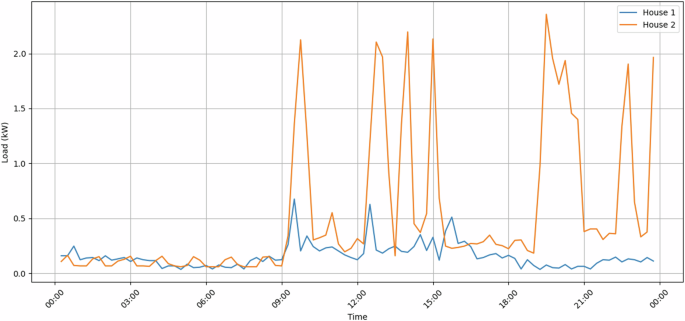
Load values for both houses 1 and 2 for the day 2021-05-01.

Full size image

Weather

For the weather information, we obtained one file per house location. Table 5 refers to the variables included in each one of these files.

Each weather file included in our dataset has 116641 rows of data. The time interval varies from 2021-01-01 to 2024-04-30, and each sample was collected in 15-minute intervals. Figure 8 illustrates an example of solar irradiation (GHI) over time for both a sunny and a rainy day. The figure also includes a graphical representation of weather conditions, explicitly showing the cloud types to depict the sky status.

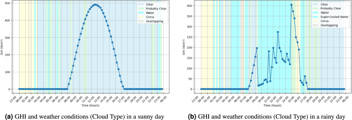
Example of solar irradiation data on days with different weather conditions in House 1.

Full size image

Market Energy Price

The Price folder contains a single CSV file with information regarding the gross market price of electricity. The file includes five features described in Table 6. This CSV has 81073 rows of data from 2015-01-01 to 2024-04-01, with entries recorded at hourly intervals.

PV Power Generation

The last part of the SHEERM dataset is the one for the PV generation associated with each house. In its folder are 13 CSV files corresponding to the generated power given the specificities of the associated solar panel. The CSV file of each house contains the following variables: Timestamp, Cos Solar Incidence (°), GHI (W/m²), and PV Power Generation (W). Table 7 briefly explains each variable.

Similar to household power consumption, Table 8 summarizes the available data for each house, detailing the quantity of data and the timespan of photovoltaic power generation.

All data in this dataset can be correlated through the timestamp, encompassing various energy-related dimensions. This comprehensive integration facilitates the creation of a holistic view of energy availability and consumption, aiding in the design of efficient, energy-integrated systems. Figure 9 illustrates the energy dimensions presented in the dataset. This approach aims to support the transition towards renewable energy and carbon neutrality.

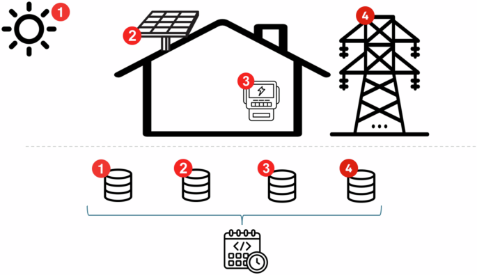
Energy dimensions included in the dataset: 1 – Weather data; 2 – Solar panel information; 3 – Household Load; 4 – Grid Price.

Full size image

Since this dataset is essential for predictive analysis and the development of prediction models, the technical validation involves building machine learning models using the data from the records to assess their suitability. The dataset features extensive, cross-sectional solar energy production data directly linked to solar irradiation, weather parameters, and specific household load requirements. Combining these features enables multifaceted analysis, fostering advancements in renewable energy forecasting, climate-sensitive environments, grid management, and energy policy formulation. This dataset aims to aid in designing new energy systems that enhance sustainable energy strategies, demonstrating their potential to accelerate the transition towards renewable energy and carbon neutrality.

As explained in the Data Records Section, the SHEERM dataset includes two sets of data for household consumption data (Load): raw and processed data. The processed set of data has no missing data or outliers. In this technical validation, we will use the processed set of data. Regarding household energy consumption, we ensure no data is missing or outliers through the data acquisition protocol and the data processing done on the server when a data sample is received. Concerning weather data, since the initial data was fetched from the NSRBD, we have checked, and there is no missing data. Regarding the new features added to the NSRBD, they were computed for all entries in the dataset, resulting in no missing data. Regarding photovoltaic energy generation data, since it was computed through Equations (1), (2) and (3), there is also no missing data associated with it.

However, suppose more data is added to the SHEERM dataset, and gaps are generated. In that case, techniques such as those used in our acquisition procedure can be used to fill those gaps. For instance, using an LSTM, the time series data can be predicted for several instances ahead. So, if there is missing data, it can filled with the predicted values generated by the LSTM. Other approaches or statistical models can also be used, such as forward or backward fill, linear interpolation, interpolation with splines or polynomial methods, moving averages, seasonal decomposition, and other machine learning techniques.

The simplest way to fill data gaps may be to use the forward or backward fill, where missing values are filled with the last known value (forward fill) or the next known value (backward fill). This technique is appropriate when consecutive data points, such as short-term missing data, are expected to be similar.

Linear interpolation techniques⁵⁰ can be used to estimate missing values by connecting the points before and after the gap with a straight line. This technique is suitable for small gaps in data where the values are expected to change linearly. Interpolation with splines or polynomial methods^51,52 is another option to fill the gaps. These techniques use polynomial or spline curves to fit the data points and use it to estimate missing values. They are useful when the data has a non-linear pattern.

Moving average techniques^53,54,55 can also fill missing values with the average of neighboring data points over a specified window. It is useful when the missing data is part of a more significant trend and smoothing is desired.

A more complex approach can also be used, like seasonal decomposition, where the time series is decomposed into trends (seasonality). Missing values can be filled by estimating from trend behavior. This method is effective when the data has strong seasonal patterns, like weather data. Lastly, similar to what we did in our acquisition procedure, algorithms like K-Nearest Neighbors (KNN), Random Forest, or even deep learning models can be used to estimate missing values^{53,56,57,– 58}. These methods are appropriate for datasets where simple methods might not capture underlying patterns. They are suitable for situations where certain weather events are known, and no statistical model can account for them.

The technical validation aims to verify that our dataset is appropriate for predicting future values for household energy consumption, weather conditions, photovoltaic energy production, and energy market price. Similar to the most relevant datasets presented in the literature (Table 1), for the technical validation, we developed various machine learning methods to conduct several analyses and demonstrate the consistency, accuracy, and usability of the provided data. These include predicting household energy needs, forecasting weather conditions, estimating photovoltaic energy production based on predicted weather conditions, and projecting trends in energy prices. These examples showcase the practical applications of the dataset and the potential insights it can provide.

The machine learning models were implemented using the Python programming language (version 3.11.6), which is supported by several Python libraries. Pandas (version 2.1.1) was employed for data manipulation and analysis, while NumPy (version 1.24.4) helped us with efficient numerical computations. The Matplotlib Python library (version 3.8.0) was also used, aiding us in creating plots for visualizing data trends and patterns. Scikit-learn (version 1.3.1) and TensorFlow (version 2.14.0) were used to implement machine and deep learning models and evaluate their performance metrics. The statsmodels library, version 0.14.0, was also used to perform the linearity analysis.

Household Consumption Data (Load)

The analysis of the household consumption data involves a linearity analysis to assess the underlying data characteristics. Then, we demonstrate the effectiveness of various machine learning models in capturing trends and accurately forecasting household consumption. This approach allows us to assess whether models can provide reliable predictions based on the data’s inherent patterns.

Linearity analysis is an important method for understanding the data and selecting the best predictive model. Since linear models are more easily interpreted and computationally efficient, linearity analysis can assess whether models like linear regression are appropriate or need more complex models. Additionally, understanding the data’s linearity may help to improve the model’s accuracy and prevent overfitting.

Based on Ramsey’s RESET test⁵⁹ and the Ordinary Least Squares (OLS)⁶⁰ regression, we designed two approaches for this analysis: 1) considering the entire dataset, where the linearity analysis is performed at once on the entire time series, and 2) considering sliding windows, where the time series is divided into smaller time frames and the linearity analysis is performed on each window separately. The first approach is simple to implement and reduces complexity. It helps identify the overall data behavior in terms of linearity but may overlook local variations of the data that do not fit the global trend. The second approach analyzes smaller data sections (106433 windows were considered), which detect local linear relationships that might not be visible in the overall dataset. This approach is beneficial in the Load data analysis since it is a time series with varying conditions, like day/night, week/weekend, and summer/winter.

Table 9 summarizes the results of our linearity analysis on household consumption data considering different sliding window sizes and the entire time series. The results show the ratio of analyzed windows whose pâ€�value  < â€‰0.05. The study suggests that the data exhibits mostly linear patterns for small window sizes. Ramsey’s RESET test shows that we can not reject the null hypothesis (i.e., the data could be modeled by a linear expression since there is no evidence to suggest that the linear model is misspecified). However, the results suggest that the linear model is misspecified for large window sizes (windows greater than 12 hours), meaning the data follows a non-linear pattern. These results suggest that traditional linear models may not effectively capture the underlying trends. Table 10 This observation highlights the need for machine learning models that are better suited to handle non-linear relationships in predictive modeling.

Regarding machine learning applicability, this technical validation focuses on creating various predictive models using LSTMs, RFR, XGBoost, and MLP algorithms to predict the load values for each house. Since the household data was acquired through certificate equipment (smart meters according to the EC Directive 2004/22/EC), the technical validation of the household data involves creating a predictive model that accurately predicts the load for the houses. We present the architecture of the LSTM model (Table 11) as well as the hyperparameters used for the RFR, XGBoost, and MLP (Table 12), noting that the architecture and the hyperparameters were chosen through applying a grid search optimization algorithm⁶¹. The grid search was conducted on the household consumption data, where various intervals of values were evaluated to enhance the model’s performance. The range of values tested for each hyperparameter is represented in Table 10.

The data split was into 75% train and 25% test applied to each household consumption data. Each model, LSTM, XGBost, MLP Regressor, and Random Forest, is trained for each one of the houses (using 75% of the data) and evaluated in the remaining 25%. We compared the real values for the load of the house and the predicted ones. The evaluation metrics used to assess each model include the root mean squared error (RMSE), Mean squared error (MSE), and R-squared (R2). Table 13 presents the evaluation metrics obtained from applying the models to their corresponding test data. All values were forecasted for a timespan of one day ahead (96 points ahead). From the results obtained, we could conclude that, on average, the model that tends to be more accurate according to R2 and leads to fewer errors is the LSTM model.

Based on the R2 results, we identify a good relation between the predicted data and the real data for the LSTM model, meaning that the data can be used to train/develop these machine-learning models and predict the energy needed. Figure 10 graphically represents some of the predicted and real values obtained for the houses for a given day, illustrating the model’s predictive capabilities and, consequently, the validity of the data.

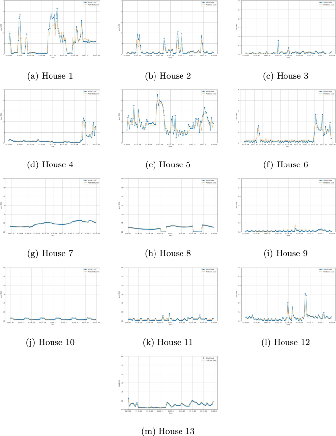
Load predictions for multiple houses using an LSTM model.

Full size image

Weather and photovoltaic power generation

For the technical validation of weather and photovoltaic power generation prediction, we used two methods. The GHI in SHEERM and a real-world experiment were compared first. Second, LSTM deep learning models are used to predict solar irradiation, and a Random Forest Classifier is used to predict cloud type.

Since the GHI was obtained from an external source (NSRDB), we looked at another dataset to validate the data. Upon an extensive search, we identified the work done by T. Yao⁶². In this work, the authors provided data for GHI in their location based on a numerical weather prediction (NWP) method⁶³. Since the NSRDB allows us to select any position in the world and fetch data for that position, we identify the locations used by T. Yao’s work and compare the data fetched from NSRDB against their NWP data.

Figure 11 depicts this comparison and shows the similarity between the NSRDB and the NWP data, which allows us to conclude that the data fetched from NSRDB is reliable. However, the data from both sources assume a tilted position of β  = â€‰0° of the solar panel, which is only valid for positions on the equatorial line at noon. Since our data was collected in the north hemisphere, a tilt angle is used in the solar panel to maximize the captured energy, which means that the GHI must be corrected to consider this influence. For that, Equation (3) is used. Considering the tilt angle of the panel β  = â€‰33°, the estimated GHI is shown through the yellow curve in Fig. 11. As we can see, the panel’s tilt angle significantly influences the quantity of captured solar irradiation. This influence is considered in our data related to the photovoltaic power generation, considering the position of each panel and its configuration.

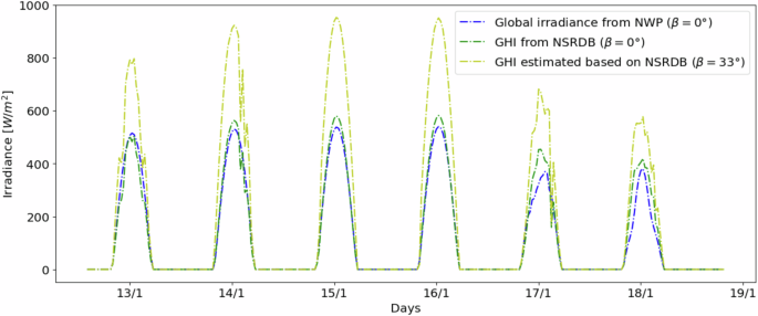
Comparison of the GHI values provided by the NSRDB and NWP considering β  = â€‰0°, and the GHI estimated based on the NSRDB considering the tilt angle β  = â€‰33° of a location from⁶².

Full size image

Tables 14 and 15 represent a summary of the weather data in the dataset per house and region, respectively. Since the outside temperature and humidity influence the efficiency of solar panels, we show these values per house and area, which can help in further analysis, allowing us to adjust the prediction model to reflect real-world conditions according to the region where the houses are.

Moreover, household energy consumption is closely related to temperature variations. Heating and cooling needs fluctuate with temperature changes, making this data vital for accurate consumption forecasting. Precipitation, cloud cover, and wind conditions can also impact solar energy production and household energy use. For instance, cloudy or rainy days might also increase indoor lighting and heating demand.

Regarding photovoltaic power generation data, as detailed in the methodology section, it was computed using Eq. (1)^45,46. To assess the reliability of the chosen model and the resulting data contained in the SHEERM dataset, we conducted a comparison between the real-world measurements provided by the Open Power System Data (OPSD) database²⁶ and the corresponding result obtained through Eq. (1). Figure 12 compares the theoretical model results and the real-world measurements. The figure reveals slight deviations between the two, which, upon closer examination, do not appear to stem from inaccuracies in the model itself. Instead, we believe these deviations are likely due to inaccuracies in the solar irradiation measurements from OPSD (i.e., the input data Δ of Eq. (1)). This conclusion is supported by the model consistently following the same trend as the real-world data, often closely matching or overlapping with the measured values. This comparison between the OPSD’s real-world measurements and the results obtained from our theoretical model provides an additional validation step. It allows us to evaluate the reliability of the photovoltaic power generation data included in the SHEERM dataset, ensuring that the theoretical model produces reliable estimations.

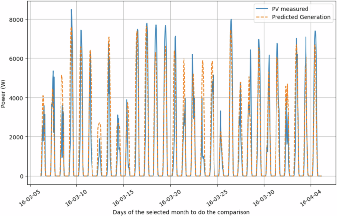
Comparison of Photovoltaic real-world measurements and theoretical model calculations.

Full size image

We also conducted a linearity analysis on the same data (weather and photovoltaic power generation data). Due to the seasonality inherent in the data, mainly the weather data propagated to the photovoltaic power generation data, the analysis revealed a non-linear trend in both sets of data. For the sake of not being exhaustive, due to the amount of weather and photovoltaic time series, the linearity test values are not incorporated in this article. Still, they can be obtained in our Jupyter notebook (see⁴⁹).

Since this work aims to contribute to the development of enhanced weather and photovoltaic perdition models, like the one used by R. Peeriga et al.⁶⁴, Y. Hao et al.⁶⁵, Z. Hu et al.⁶⁶ or F. Campos et al.⁶⁷, for this technical validation, an LSTM is used to demonstrate the usability of the weather dataset. This example involves developing an LSTM to predict the Global Horizontal Irradiance (GHI). Moreover, evaluating a predictive model for GHI values and predicting the Cloud Type is necessary since both can provide deeper insights into the data.

Predicting two main variables, GHI and Cloud Type, are important for determining the solar power generated by a solar panel. Specifically, an LSTM model with the architecture shown in Table 16 was applied to each house to predict GHI, using an 80% training and 20% testing data split. This architecture resulted from a grid search approach, where the range of values tested for each hyperparameter is presented in Table 10.

Regarding cloud type prediction, it is important to accurately determine solar irradiation and, consequently, the solar power generated. Different cloud types have distinct effects on solar irradiation. Some may diffuse or block sunlight more than others, leading to significant variability in the amount of solar irradiation that reaches the solar panel surface. Predicting cloud types allows us to model these variations more precisely, significantly enhancing the accuracy of solar irradiation predictions. This reassures us about the reliability of the data we are working with, making our predictions more robust.

In the context of machine learning, segmenting the problem first to predict cloud types allows us to design more reliable prediction models. This enables us to account for the specific influence of various cloud formations on solar irradiation. For example, high-altitude clouds might partially block sunlight, while dense clouds could significantly reduce solar irradiation. By incorporating this information into our models, we can enhance the predictive performance of solar power generation models, leading to better forecasting systems. Due to its categorical nature, a random forest classifier (RFC) was used to predict the cloud-type variable. The model architecture used comprises n_estimators = 90, max_depth = 22, and random_state = 2024.

From both the LSTM and the RFC models, the evaluation metrics are represented in Table 17. Additionally, Figs. 13 and 14 represent the predicted and real values for both the GHI and Cloud Type. Figure 14 emphasizes the influence of the clouds in the GHI by overlapping both representations. The obtained results show that the predictions for both the GHI and the Cloud Type are good, demonstrating the data’s usability and accuracy.

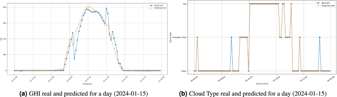
Weather’s data.

Full size image

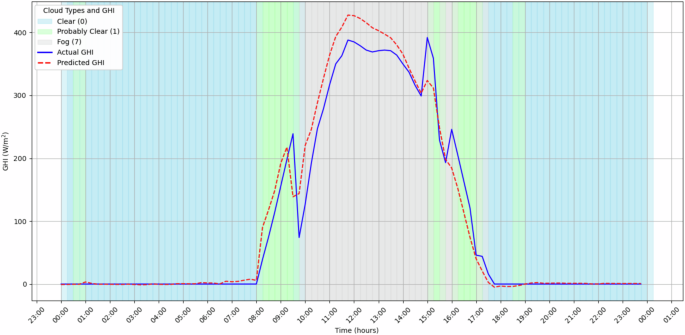
GHI real and predicted with the predicted Cloud Type for a day (2024-01-15).

Full size image

Market Energy Price Data

In this section, we used the same four machine learning models (LSTMs, RFR, XGBoost, and MLP) to predict household consumption and the gross market price of electricity. The same architecture and hyperparameters for RFR, XGBoost, and the MLP were applied (see Table 12). Concerning the LSTM model, since the energy market price series shows a smoother trend, a new architecture with the configuration represented in Table 18 was applied. Regarding the amount of data used to train and test, the same data portions were used as before (train = 75%, test = 25%).

The Ember-climate dataset provides a comprehensive overview of market prices across the European Union, ensuring that our data is reliable and up-to-date.

The first thing to note is that the prediction is only applied to the values after 2021. Before this date, the values for the price were relatively uniform and did not show any significant changes. However, after 2021, there has been a substantial change in the distribution of values. It is best to apply our model only to that section to better understand the model’s capabilities. To perform this analysis, data from 2021 to 2024 was used for training, and data from the last year was used for prediction.

From the obtained results (Table 19), it is possible to conclude that the model performs better in the LSTM even though all results are very satisfactory. This performance allows us to conclude the SHEERM dataset is reliable and can be used to aid in designing new energy systems that enhance sustainable energy strategies.

Figure 15 compares the actual and predicted energy market prices for a specific day (2023-10-11) forecasted by using the LSTM model. The figure shows a slight deviation between the predicted and real values, with the predictions being slightly lower. This indicates that our predictive model is not fully calibrated and requires further refinement. However, we assume the data is reliable for this validation since the predictions follow the same pattern as the actual values. Moreover, Table 19 shows the values for the evaluation metrics, reinforcing the idea that there are no problems with the data.

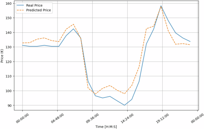
Real and Predicted values for House 1 for a specific day (2023-10-11).

Full size image

We also analyzed linearity using the market energy price data from the SHEERM dataset. By applying the sliding window approach, we identified windows where linear models may be appropriate, particularly for short-term price forecasting during stable periods. However, the analysis confirms that energy prices are predominantly non-linear, driven by shocks, seasonal patterns, and regulatory interventions. Consequently, non-linear models may be more effective for capturing the dynamics of energy markets. The linearity test values can be obtained through the Jupyter notebook we provide (see⁴⁹).

Data Correlations

Understanding and analyzing data correlations is fundamental to identifying dataset patterns and dependencies. In the SHEERM context, this analysis allows for an understanding of how variables are correlated with energy consumption behavior. Based on this knowledge, we can enhance the accuracy of predictive models, identify potential causative factors, and inform optimization strategies. This section analyzes the possible correlations presented in the SHEERM dataset. For this analysis, two houses in different regions were selected as case studies. Specifically, houses 1 and 3 were chosen as representative examples.

We first explore the relationship between household energy consumption and external temperature (Fig. 16). This analysis helps determine how much household energy usage is driven by heating or cooling demands, providing insights into how external temperature influences energy consumption behavior.

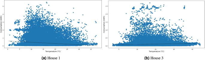
Correlation between household load consumption versus temperature.

Full size image

As shown in Fig. 16, each house exhibits distinct energy consumption patterns. House 1’s trend indicates that energy consumption tends to increase as temperatures decrease. In contrast, House 3 shows the opposite trend, also with higher energy consumption observed at higher temperatures. These differences can be due to the houses’ locations. They are located in different regions of Portugal, with House 1 in the central coastal zone while House 3 is in the center of Portugal. Typically, in the center of Portugal, heating systems are predominantly fueled by wood, meaning their energy usage is not reflected in household electrical consumption. Contrarily, cooling systems, especially air-conditioning units, rely on electricity, leading to higher energy consumption during warmer temperatures. House 1, located in a region with milder temperature fluctuations and where wood-based heating systems are uncommon, demonstrates a different pattern. Here, household electrical consumption tends to increase during freezing temperatures due to the dependence on electric heating systems.

Regarding the correlation between household energy consumption and energy market prices, Fig. 17 illustrates their relationship and the corresponding trend line. Upon analyzing the trend line, it becomes evident that it has an insignificant slope, indicating that household energy consumption is independent of oscillations in energy market prices for these houses.

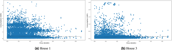
Correlation between household load consumption versus energy market price.

Full size image

Additionally, we depict the correlation between photovoltaic power generation capacity and solar irradiance. As shown in Equation (1), the power output of solar panels is directly proportional to the irradiance they receive. Figure 18 illustrates this relationship.

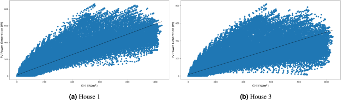
Correlation between photovoltaic energy production and global horizontal irradiance.

Full size image

As an example of using our data, we selected several machine learning methods commonly used in related work to determine the most suitable one for predicting outcomes based on weather and household load data. Five models (Support vector regression (SVR)⁶⁸, random forest regression (RFR)⁶⁹, eXtreme Gradient Boosting (XGBoost)⁷⁰, Multilayer Perceptron (MLP)⁷¹, and Long Short-Term Memory (LSTM)⁷²) were used. Only data from house 1 was used, and it was split into training and test sets (70% and 30%, respectively). The models were evaluated according to the following metrics: Mean Squared Error (MSE), Root Mean Squared Error (RMSE), Mean Absolute Error (MAE), and R-squared (R2).

For this usage example, we combined the weather information with the load data for house 1, and a test was conducted to determine the most effective feature selection method. In the related work, two prominent methods, Principal Component Analysis (PCA)⁷³ and Pearson’s correlation matrix⁷⁴, emerged as notable choices. However, to apply Pearson’s correlation, the data must meet the Pearson Correlation assumptions, such as approximating a normal distribution and exhibiting linear relationships. We conducted a preliminary evaluation based on inspecting scatter plots to confirm the linearity of variables such as GHI and DHI and using histograms to verify if the data follows a normal distribution.

Then, these two methods were tested for feature selection, with the target variable being the solar energy obtained from the solar panel. The results were also compared with the dataset containing all the features after their removal to assess significant differences when applying the feature selection methods. Both PCA and Pearson’s correlation used a threshold of 0.1, indicating that the features needed to explain 0.9 of the variability.

The results led to the creation of two subsets of data: one for PCA and the other for Pearson’s correlation, resulting in the following features for the PCA (subset 1): ’Month’, ’Day’, ’Temperature’, ’Cloud Type’, ’Dew Point’, ’DHI’, ’DNI’, ’Fill Flag’, ’Ozone’, ’Relative Humidity’, ’Solar Zenith Angle’, ’Surface Albedo’, ’Pressure’, ’Precipitable Water’, ’Wind Direction’, ’Wind Speed’, ’Energy (kW)’. After applying Pearson’s Correlation, the most representative set of features (subset 2) is reduced. It includes: ’Temperature’, ’Cloud Type’, ’DHI’, ’DNI’, ’Relative Humidity’, ’Solar Zenith Angle’, ’Surface Albedo’, ’Wind Speed’, ’Energy (kW)’. Then, each machine learning model was applied to the three sets of data: subset 1, subset 2, and the full dataset (subset 3). All models were defined using libraries such as Keras⁷⁵, XGBoost^76,77, and Scikit-learn^78,79.

To optimize the models, hyperparameter tuning was applied to explore potentially better parameters for improved forecasting. The Optuna library⁸⁰ facilitated this process, offering enhanced hyperparameter search capabilities. The specific hyperparameter ranges for each model are detailed in Table 20. Upon applying all the models and configurations, Table 21 shows the results for each model and subset of data.

Based on the results, we can see good performance across all subsets of data. All models show a low MSE, RMSE, and MAE, meaning the model predicts accurately. This indicates that the data is consistent and reliable enough to be used by machine learning models. Additionally, high R-squared values, close to 1, indicate a very good fit of the model to the data. Again, this demonstrates the usability of the data.