A suitable housing environment is needed to maintain the welfare of pigs and protect the health of farm workers. In intensive pig production, the main environmental factors that affect the growth and health of pigs are temperature, humidity, carbon dioxide (CO₂) and ammonia (NH₃) concentrations in pig houses^1,2,3,4. Temperature, one of the most important external environmental factors maintaining the body temperature of pigs at a constant level, affects the health level and reproduction ability of pigs, and directly impacts their heat balance⁵. The humidity in the pig house also affects the body heat regulation of pigs. A high-temperature and high-humidity environment decelerates the growth of pigs, and increases bacterial growth that can lead to diseases⁶. A high NH₃ concentration in the pig house can affect the growth of pigs, leading to a decrease in immunity and productivity, and inducing respiratory diseases. In addition, NH₃ emitted from pig houses can also cause pollution to the surrounding environment and increase the risk of respiratory diseases to farm workers and neighboring residents⁷. Carbon dioxide is mainly produced from pig respiration. High CO₂ concentration in pig houses not only causes dizziness and decreased production, but also harms the life of pigs⁸. Therefore, research into advanced prediction models of livestock housing environments is essential to improve animal welfare, protect the health of farm workers, and promote environmental sustainability.

Currently, the prediction models for confined environments such as greenhouses and poultry houses are mainly divided into mechanism models and data models^9,10. A mechanism model acts as an environmental prediction model by considering the interactions between factors based on principles such as conservation of energy and mass. Xie et al.¹¹ established a dynamic prediction model of heat and humidity in a pig house based on the equations of energy and mass balance, and determined the model parameters by combining them with the measured data, thus predicting the changing rules of temperature and humidity in the pig house. Cooper et al.¹² developed a steady-state model based on heat balance analysis, and combined it with natural ventilation, thermal buoyancy solar radiation, and other factors to predict the average hourly temperature inside livestock and poultry buildings. Zhao et al.¹³ built a steady-state numerical model to predict ventilation and heat load in caged laying hen houses, and used it to optimize environmental conditions in the hen house and management programs. Wang et al.¹⁴ constructed a new ventilation system model to achieve the required temperature and humidity environment for growth in a hen house by controlling the amount of ventilation. However, the predictive performances of these methods are unstable and affected by the type and accuracy of the input data, the structure of the actual livestock and poultry house, and unknown parameters in addition to high costs and complex modeling.

Data models are mainly based on machine learning and deep learning to train and test datasets without considering the influence of physical properties, and can be built directly from the data^{15,16,17,18,19}. Machine learning models include decision trees, support vector machine, support vector regression, and least square support vector machine^{20,21,22,23,24}. Machine learning models can capture non-linear relationships in temporal data to a limited extent. However, machine learning is limited by long training time, poor generalization ability and complex structures, making it unable to adapt to large temporal data. Deep learning-based models can more effectively use the data and fully explore the linear and nonlinear features hidden in spatiotemporal sequence data. Xie et al.^25,26 established a well-fitting ANFIS prediction model using five types of membership functions and an NH₃ emission prediction model based on the NH₃ concentration of fattening pigs. Zang et al.²⁷ developed an integrated empirical mode decomposition gated cyclic unit (GRU) model to predict carbon dioxide concentration in pig houses. Peng et al.²⁸ selected three traditional machine learning algorithms and three deep learning algorithms to predict ammonia concentration in pig houses, and found the hybrid prediction model had higher accuracy. Ji et al.²⁹ proposed a multi-stage environmental prediction model based on the long-term short-term memory (LSTM) and Informer in rabbit houses, which effectively improved the prediction accuracy of temperature and humidity in rabbit houses. Guo et al.³⁰ predicted the ammonia concentration in chicken houses based on a two-stage attention-recurrent neural network (RNN) and LSTM algorithms, and predicted the trend of ammonia concentration in chicken houses. Guo et al.³¹ proposed an environmental prediction model based on osprey adaptive t-distribution dung beetle optimization—temporal convolutional network (TCN) -GRU for pig houses, which improved the accuracy and stability of predicting environmental conditions in pig houses. Although the different types of models show their respective advantages in animal husbandry environments, they have certain limitations.

To address these challenges, a prediction model of a pig house environment based on the Bayesian optimization (BO) algorithm, squeeze and excitement block (SE), convolutional neural network (CNN), and GRU is proposed. In this model, a probability agent model based on BO is built to sample the objective function and to find the optimal hyperparameter combination. The SE module adaptively recalibrates features according to the importance, which improves the ability of CNN to extract abstract spatial features. Moreover, GRU can effectively capture long-term dependencies in time series. Such combination makes the BO-SE-CNN-GRU prediction model deal with the variability of pigsty data, and improves the prediction accuracy of time series. The prediction accuracy is significantly improved by implementing the BO-SE-CNN-GRU model, which provides scientific decision support for fine-grained supervision of pig houses.

Data acquisition

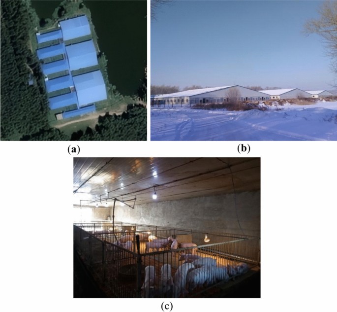
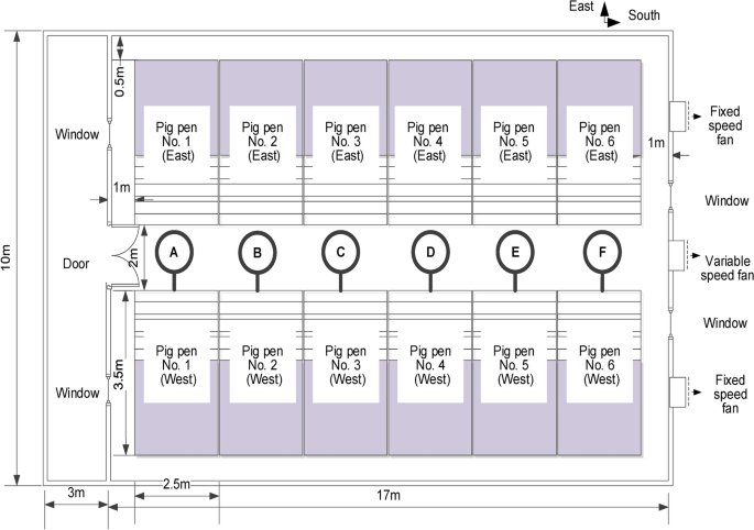
The environmental parameters of the experimental pig house were collected from a nursery pig house in Jianhua District, Qiqihar City, Heilongjiang Province (47°44’N, 124°04’E) (Fig. 1). The experimental pig house is 17 m long, 10 m wide and 3 m high. The south wall has two windows measuring 1.75 m long by 1.35 m wide. There are two fixed-speed fans and one variable-speed fan. The north side, which leads to the corridor, has a doorway measuring 2.1 m long by 1.2 m wide, and two windows of the same dimensions as the south side. Figure 2 shows the layout of the pig house, with A-F showing the sensor arrangement locations. The pig house consists of 12 pens, each with an area of 8.75 m². Six and six pens are located symmetrically on the east and west sides respectively. Each pen houses 10–12 nursery pigs with an average weight of 12 kg. The standing height of nursery pigs is about 0.4 m and the lying height is about 0.2 m.

Indoor environmental data were collected using an environmental monitoring system (Shandong Weimengshi Technology Co., Ltd., China). The parameters of the sensors used are shown in Table 1. The data collected include indoor and outdoor temperature and humidity, carbon dioxide and ammonia concentrations. The sensor monitoring nodes were mounted in the west pens of the pig house and at a height of 0.2 m above the ground. An environmental prediction model was built using the average values of the environmental parameters measured at six points. The outdoor temperature and humidity were recorded by a small weather station in the surrounding area. From 11 December 2022 to 14 January 2023, all sensors collected data every 15 min, for a total of 8730 pieces of data.

Data processing

Processing of missing data

Sensors can be affected by the hardware condition and the complex environmental factors in pig houses, which is a significant challenge to data collection. In addition, issues such as network transmission quality and mechanical failures can result in inaccurate or missing data. To make the time series of the dataset complete for further processing, the missing data must be interpolated and filled.

Any data collected over a certain time interval is a time series. The data sets of the collected environmental parameters are also time series, and are an organized collection of periodically measured values. Therefore, a linear interpolation algorithm is used to estimate the missing data points by using the surrounding data:

where TS_{i, n} is defined as the n-length time series of an environmental parameter. The sampling interval for all data is 15 min, meaning all parameters are measured at the same time each day. If the value X_i,b at T_b is missing, it can be approximated using a linear interpolation algorithm as follows:

When the environmental parameters are lost at any time, the algorithm first finds the two closest times, denoted as T_a and T_c. Then the missing values at time T_b are calculated using the parameter values X_i,a and X_i,c at time T_a and T_c, respectively, according to Eq. (2), where X_i,b is the estimated value of the missing value X_i,b.

Data normalization

Data are normalized to eliminate the effect of data size in different dimensions on the predictive model and to improve model performance. Specifically, the features among different dimensions of a dataset on the same dimension are compared, eliminating feature differences across dimensions and orders of magnitude. Normalization methods include linear function normalization and zero mean normalization. The original data are linearly transformed using the maximum and minimum normalization method to improve the convergence speed and prediction accuracy of the model³²:

where X_i is the value before normalization, X_min and X_max are the minimum and maximum values in the same variable, and X_norm is the value after normalization.

Structure of the proposed model

SE-CNN-GRU model

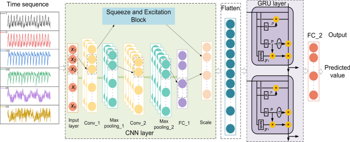
This study proposes a neural network prediction model that combines the automatic tuning of model hyperparameters of the BO algorithm, the feature enhancement of SE-CNN, and extraction with GRU learning of time-dependent relationships. The structure of the model is shown in Fig. 3.

The model prediction process is elaborated below. First, the monitored environmental data (e.g., indoor temperature, indoor humidity, carbon dioxide concentration, outdoor temperature, outdoor humidity) are input into the model. The BO algorithm optimizes the model hyperparameters, including the number of neurons in the GRU, the initial learning rate, and the L2 normal form regularization. The combination of parameters is optimized to improve the prediction accuracy of the model. The environmental data are input to the SE-CNN block, which extracts the local features of the data through convolution operation. The SE block further learns the weights of the feature channels, highlighting the important features and suppressing the unimportant features, and thus improves the discriminative ability of the features. The local features extracted by the SE-CNN are fed into the GRU network to capture the long-term dependencies in the sequence, and this information is used to predict future values. The extracted features of the SE-CNN are connected to the GRU output and predicted through the fully-connected layer to predict the final values of the indoor environmental parameters. The model can dynamically adjust the importance of different input signals within the model according to the environmental data, resulting in more accurate predictions.

CNN based on attention mechanism

CNN is a feedforward neural network that exploits features such as local connectivity and shared weights^33,34. The CNN uses convolutional kernels of different sizes to extract deep spatial features from raw data, thereby reducing dimensionality. We use a CNN model to capture these features from our dataset. A CNN model typically consists of several layers, including convolutional and pooling layers. The operation in the convolutional layer is shown as:

where C is the feature output after the convolution operation, f( ) is the Relu activation function, X is the input data, ∗ is the convolution operation, W is the weight of the convolution kernel, and B is the additive bias.

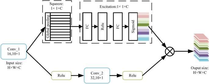
To improve the feature extraction performance and environmental data prediction accuracy, channel attention SE block is used to recalibrate the deep feature maps extracted by CNN. SE block with squeeze and excitation operations can automatically learn global information and assign different weights to the filtering channels, selectively focusing on important features and reducing redundant information. The schematic diagram and working principle of SE block are shown in Fig. 4.

The CNN structure combined with the SE block is shown in Fig. 5. The SE block, located after the CNN network, uses the SE block to improve the feature representation of the channels. The feature representation is enhanced by emphasizing on important features and suppressing irrelevant features. The SE block allows the network to focus on the most informative features by selectively increasing the weights of channels that contribute significantly to the classification and decreasing the weights of less relevant channels³⁵. This selective weighting process ensures that the network effectively extracts discriminative information and thus improves accuracy.

For a given input image X of size (H’, W’, C’), it can be mapped onto a feature map U where U ∈ R^{H×W×C} by a set of convolutional transformations F_tr as described in section A³⁶. The output U = [u₁, u₂, …, u_C] can be expressed as

where * denotes the convolution operation; V = [v₁, v₂, …, v_C] indicates the learned convolution kernels, and v_C = 

[(v_c^1v_c^1),(v_c^2v_c^2), …, (v_c^c^primev_c^c^prime)] is the C-th 2D spatial filtered kernel; X = [x¹, x², …, x^C’] and u_C ∈ R^H×W.

This step extracts global channel-wise information through global average pooling on the feature maps. This step reduces each spatial feature map into a single scalar value, representing the importance of that channel. Its mathematical expression is as follows:

where z_c is the data resulting from the squeeze operation F_sq with the data input into channel c; u_c is the channel c data of the input data.

The squeezed information is then fed into a fully-connected network, which generates weights for the channels. These weights are used to scale the original feature maps, effectively recalibrating the features based on the importance. The mathematical expression is shown as follows:

where s is the output of the excitation operation F_ex; W₁ is a layer that reduces dimensions according to the ratio r; W₂ is a layer that re-increases the data dimensions according to r.

GRU model

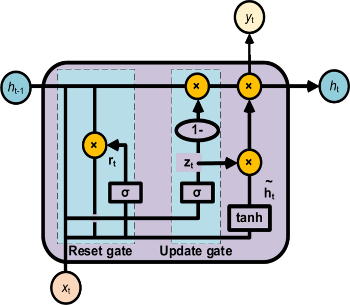
GRU is a special type of RNN with enhanced feature extraction capability in processing sequential data, thanks to its gating mechanism and recursive structure. GRU networks simplify the structure of LSTM by merging the three gates in LSTM into two gates (the update gate and the reset gate), and by combining the unit states and outputs into a single state^37,38. The structure of GRU is shown in Fig. 6. GRU can capture the dependencies on different time scales, fully exploit the intrinsic features of the time series, and solve the gradient explosion problems in RNNs. A GRU cell can be defined as:

where z_t is the update gate (0–1), σ is the sigmoid activation function, W_z is the update gate weight, x_t is the input, h_t−1 is the activation value at the previous time, r_t is the reset gate specifying how the previous state information is combined with the new input information, W_r is the update gate weight, tanh is the tanh activation function, (widetildeh_twidetildeh_t) is the hidden state information of the current time, and h_t is the output value at the current time.

Bayesian optimization

The performance of a deep learning model is critically dependent on the optimal choice of hyperparameters, such as neuron number, learning rate, and batch size. Traditional methods such as grid search and random search often struggle with efficiency, especially when dealing with a large number of hyperparameters³⁹. For example, grid search requires significant computational resources, owing to its exhaustive exploration of the search space. While random search is more efficient, it may not be as effective as Bayesian optimization, a technique that uses intelligent optimization algorithms^40,41.

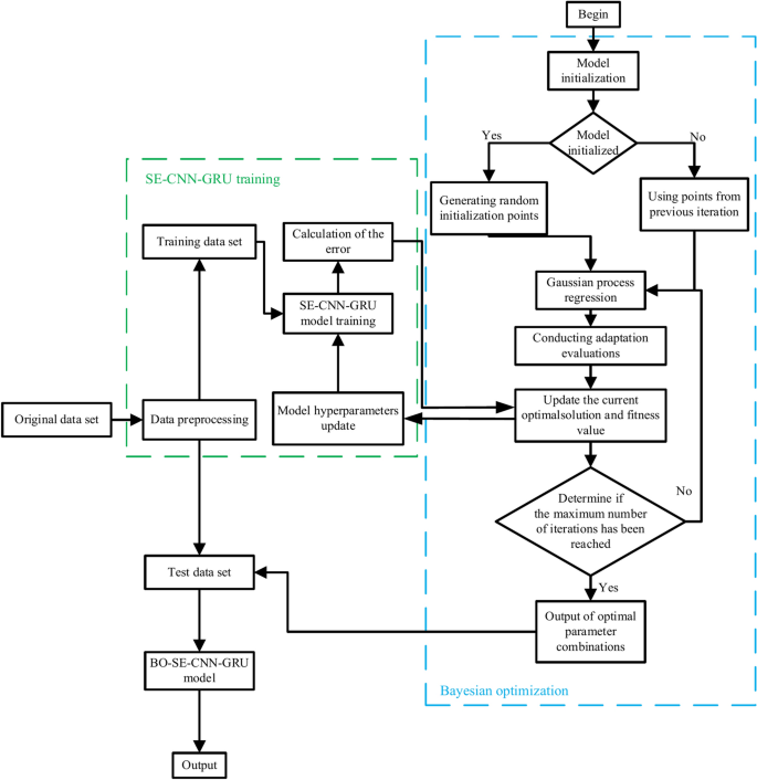
Bayesian optimization is a global optimization method that seeks the optimal solution for an objective function, and is mainly used to find the global optimal solution for complex black-box functions⁴². The core of Bayesian optimization is to use a Gaussian process regression to model the objective function, and the prior knowledge is used and iteratively updated as per the observed data to efficiently search for the optimal solution. The Bayesian optimization algorithm constructs an agent model of the objective function, and incorporates a sampling function to guide the sampling process. The function prioritizes points with a high probability of improvement over the current best observation. The advantage of Bayesian optimization is that it can find the optimal solution using the minimum numbers of iterations and computer resources. It also can construct alternative models to approximate the relationship between the objective function and the hyperparameters, and thus identifies the optimal solution of the unknown objective function. It updates the hyperparameters sequentially to find the best hyperparameter combination.

Root mean square error (RMSE) is used as the objective function for Bayesian optimization. Bayesian optimization uses previous sampling points to predict the shape of the objective function, and guides the search process by selecting sampling points that are more likely to find improvements than the current best observation. It finds the point where the hyperparameter value can derive the maximum result expected by the user. Figure 7 shows the flowchart of the Bayesian algorithm for SE-CNN-GRU optimization. In this study, we integrated the BO algorithm to optimize various parameters, including number of neurons in second GRU, the initial learning rate and L2 normal form regularization.

Model performance evaluation

The accuracy and predictive ability of the model are measured using the coefficient of determination (R²), the mean absolute percentage error (MAPE), and the mean absolute error (MAE). Larger R², smaller MAPE and MAE mean the model has better predictive ability. The model evaluation indexes are shown in Eqs. (12)–(14), respectively:

where N refers to the total number of data, x_i is the true value, and (widehatx_i widehatx_i ) is the predicted value.

Data analysis

The dataset for the experiment comprises indoor temperature, indoor humidity, outdoor temperature, outdoor humidity, and of CO₂ and NH₃ concentrations, amounting to totally 8730 data points. The environmental data measured in the pig house were processed and analyzed (Table 2).

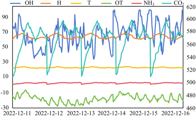
The line graphs in Fig. 8 visualize the fluctuation variables of the pig house over five days.

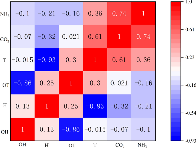
The environmental variables in the pig house are highly periodic (Table 2 and Fig. 8). Temperature first fluctuates in the opposite direction to relative humidity, and then the two variables fluctuate in a very similar way. Pearson correlation coefficients were calculated using the data of environmental variables on the first day. The calculations are summarized in Fig. 9.

The different colors in Fig. 9 indicate the degree of correlation, with darker red and darker blue indicating stronger positive and negative correlations respectively. With ammonia concentration as an example, the Pearson correlations in the changes of ammonia concentration with temperature, humidity and other factors in the pig house were calculated. Then the data that mostly severely influenced ammonia concentration among the non-time series data were judged to select the appropriate data for input and prediction. The environmental factor that has the greatest impact on ammonia concentration is CO₂ concentration, followed by indoor humidity and outdoor humidity. CO₂ concentration was negatively correlated with outdoor humidity and indoor humidity, indoor temperature and indoor humidity, and outdoor temperature and outdoor humidity.

Model optimization and training

The dataset is divided into training and testing subsets at a ratio of 7:3. The experiments are run with 500 epochs and a batch size of 128 for training and testing. A 5-parameter input and a single-parameter output prediction model is constructed to predict temperature, humidity, and CO₂ using separate output layers. Each parameter is predicted in turn. The initial parameters of the model set up in the experiment are shown in Table 3.

Optimized hyperparameters can significantly improve model performance on both training and unseen data. To more accurately model the prediction of pig house environment, optimized hyperparameters are selected using Bayesian optimization, including number of GRU neurons, initial learning rate and L2 normal form regularization. Predicted values and losses are calculated using the initial parameter values. The objective function of the Bayesian optimization is used to determine the optimized hyperparameter values. Table 4 shows the search space of the hyperparameters.

The training data of adjusting the parameters under the number of iterations are recorded, and the number of iterations is terminated to derive the final fitness. The optimization process is shown in Table 5. The Bayesian optimization algorithm quickly reaches the convergence point and the minimum value of the loss function at 27 training rounds. The application of Bayesian optimization to this model is successful. The hyperparameters of the optimization model are shown in Table 6.

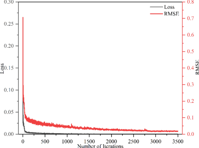
The loss and RMSE curves in the training of the proposed model are shown in Fig. 10. As the number of iterations increases, the loss and RMSE both decrease significantly and stabilize. The loss and RMSE decrease rapidly in the first 250 iterations, meaning the model learns quickly from the data. As the number of iterations increases, the loss stabilizes around 0 after almost 750 training iterations. Moreover, the RMSE decreases after 1500 iterations, and gradually stabilizes at 0.04. This result indicates the model is gradually improved without overfitting during the learning, and therefore has a strong generalization and prediction ability on the data.

Comparison of true and predicted values

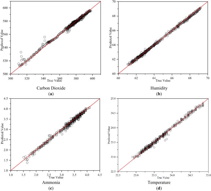
Figure 11 shows scatter plots of the predicted values from the BO-SE-CNN-GRU model against the true values. On the scatter plots, most of the points are on or near y = x, indicating the predicted values of this model are mostly very close to the true values. This trend suggests the predictions of the model are very accurate. The point distribution shows the proposed model has the highest concentration of points on y = x for humidity prediction, followed by temperature. For humidity predictions, the highest concentration of points on y = x is predicted with a maximum relative error of 0.6%, followed by temperature (0.4%). In contrast, the prediction points for CO₂ and NH₃ are more scattered and slightly less effective. The maximum relative error is 4% for CO₂ and 9% for NH₃. The prediction performance of the model is better for temperature and humidity and slightly worse for hazardous gases. In addition, the BO-SE-CNN-GRU model predicts a better response to environmental changes and yields more accurate results.

Comparison of model performance

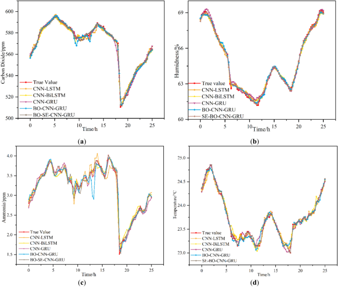
Figure 12 compares the prediction errors of environmental prediction models, such as CNN-LSTM, CNN-BiLSTM, CNN-GRU, BO-CNN-GRU, and BO-SE-CNN-GRU. The overall predictions are better for both temperature and humidity. The reason is that the pig house is an enclosed environment and the indoor temperature is more stable and less variable. CO₂ and NH₃ concentrations in the pig house are influenced by temperature, relative humidity, and external factors such as feeding practices. Hence, the variations in CO₂ and NH₃ concentrations are much severer than those in temperature and humidity. Therefore, the generalizability of each model is highly expected, and the predictions for CO₂ and NH₃ differ significantly. The CNN-LSTM and CNN-GRU models generate poor predictions, while the CNN-BiLSTM and BO-CNN-GRU models have better overall fitting. However, when predicting NH₃ during environmental mutations, the prediction accuracy of CNN-BiLSTM and BO-CNN-GRU decreases significantly and the prediction errors increase. These gases are predicted to be influenced by current conditions, but also by historical trends and patterns. The BO-SE-CNN-GRU model combines the global optimization capability of the BO, the feature recalibration capability of the SE block, the spatial feature extraction capability of the CNN, and the time-dependent learning capability of the GRU so that the model can deal more effectively with the complexity and variability of environmental data from pig farms. The architecture of the BO-SE-CNN-GRU model is suitable for capturing these non-linear relationships and patterns to derive more accurate predictions. Based on the above analyses, the BO-SE-CNN-GRU model is more accurate and predicts results closer to the actual data of the pig house environment.

The above analyses show the BO-SE-CNN-GRU model has the best predictive effect. To accurately measure the improvement of this model over several other models, R², MAPE, and MSE are used to compare model performances (Table 7). The R² is between 0 and 1, and R² closer to 1 indicates the model better fits the data. A value closer to 0 means the model fit is poorer. MAPE and MSE can quantify the amount of errors in the model predictions. The smaller MAPE and MSE suggest the prediction error of the model is smaller and the model performance is better. The comparison results show the BO-SE-CNN-GRU model has the smallest error between the predicted and actual values, the smallest MSE and MAPE, and the largest R². The results indicate the BO-SE-CNN-GRU model can more accurately explain the variation of the actual data.

In predicting temperature and humidity, the BO-SE-CNN-GRU model has better predictions with smaller increase in MSE, MAPE, and R₂ compared to other models. For example, the prediction of ammonia concentration shows a 65% reduction in MSE, a 48% reduction in MAPE, and a 3.9% improvement in R² compared to the CNN-LSTM model. The BO-SE-CNN-GRU model can capture the non-linear relationships and complex patterns of the data, more accurately predicts the target variables, and performs better in reducing prediction errors. Therefore, it can better predict the target variable than other models. In terms of the current farming needs, the model accuracy meets the decision-making needs for environmental control of pig houses.

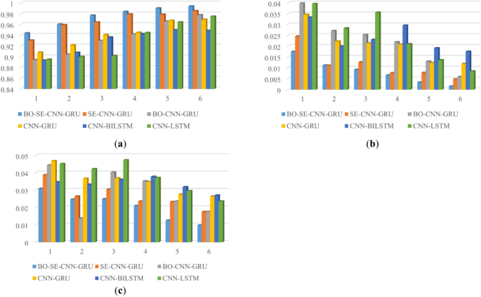
To further analyze the performances of these models, the dataset size can lead to large differences in the performance of the trained models, due to the different data distributions in the dataset. Therefore, without changing the original temporal order of the dataset, all-time series data of the pig house environment except the test set are equally divided into n consecutive equal parts. The 1st to the ith equal data (i = 1… n-1) are selected as the training set, and the (i + 1)th aliquot is the test set. The performance of the model on different parts of the data is evaluated, and overfitting is reduced by considering temporal correlations. To fully use the dataset and avoid too many calculations, NH₃ is used for analysis and n is set to be 6.

The proposed hybrid deep learning model outperforms the remaining deep learning models in terms of R², MSE and MAPE in six experiments (Fig. 13). The performance of the CNN-GRU model with embedded SE block outperforms the BO-CNN-GRU model (Fig. 13 and Table 7). The reason is that the embedding of SE makes the CNN more effectively extract features, compensating for the information loss defects of the pooling layer in the CNN and improving the generalization ability of the model. This hybrid deep learning model further improves the CNN-GRU deep learning model, combines the automatic optimization of Bayesian optimization algorithm and SE module to improve the extraction of feature information, and improves the prediction accuracy. Compared with different models, the BO-SE-CNN-GRU model has better performance with higher accuracy and robustness.

A novel pig house environment prediction model that incorporates Bayesian optimization, squeeze and excitation block, convolutional neural network and gated recurrent unit is proposed. Bayesian optimization is applied to the model to efficiently optimize hyperparameters, which significantly improves the prediction accuracy and generalization ability of the model. The feature extraction ability of the model is enhanced by adding the SE block to the CNN, which enables the model to automatically identify and predict the most relevant environmental features and improves the prediction accuracy. The GRU network effectively captures the time-dependency of the environmental parameters and maintains the stability of the prediction, even in the face of a complex dynamic environment. The environmental prediction effectiveness of various models and methods is evaluated by comparing them. Compared with other models, the BO-SE-CNN-GRU model has higher R², lower MSE and MAPE in predicting temperature, humidity, carbon dioxide and ammonia concentrations, indicating the model can more accurately reflect the trend of the real environment. It provides useful decision support for regulation of the pig house environment, protects pig health and improves production efficiency.