Environmental problems arise from the complex interactions between human activities and Earth’s systems (Lu and Guo, 1998). These interactions are key to studying sustainable development, which has become a major global research issue in the 21st century and a priority for countries and academic fields worldwide. To better understand and address these issues, scholars have developed methods to analyze spatial coupling between human economic activities and the natural environment, focusing on how human actions impact the environment and how environmental changes, in turn, respond (Steffen et al., 2015; Keeler et al., 2019; Liu, 2020). To quantify human impacts on the natural environment, classic methods such as social-ecosystem dynamics, ecosystem services assessments, and environmental footprint analysis are commonly used (Matustik and Kociv, 2021; Xu et al., 2024). Geography also supports scientific research on these environmental challenges, offering valuable theoretical frameworks, data, and technological tools. For instance, the “Future Earth Program� emphasizes the link between global environmental change and human well-being, highlighting the need to assess environmental governance and management strategies across different sectors and scales (Qu et al., 2015). In this context, economic geography can help explain the driving mechanisms behind environmental pollution, particularly through an input–output method that examines the flow of resources and waste in economic systems (Bicger et al., 2023; Chen et al., 2023). By understanding these dynamics, we can better identify the key drivers of environmental change. Additionally, its unique policy analysis methods can help formulate more effective strategies for pollution control and guide the management of natural resources to address ecological challenges (Hanink, 1995; Deacon et al., 1998).

Analyzing the spatial heterogeneity of environmental pollution from the perspective of pollution sources offers an interesting approach that integrates environmental science and geography. Pollution exhibits significant spatiotemporal variation, with sources typically following specific spatial patterns, known as environmental pollution sources, that can vary in type (Jiang et al., 2023; Zadjelovic et al., 2023). By systematically identifying and quantifying these sources and enhancing monitoring at finer spatial scales, we can better understand the causes of environmental stress. Advanced pollution tracking technologies enable precise, real-time monitoring, but receptor data may sometimes include natural diffusion residues, making it necessary to analyze pollution source structures in detail. This process typically involves statistical methods like geostatistics and principal component analysis to identify pollutant components. Bayesian inference is then used to pinpoint the primary sources of pollution and map their spatial distribution (Gupta et al., 2017; Stanimirova et al., 2024). Quantitative analysis often involves measuring emissions of specific pollutants, either total, per capita, or localized, under various social and economic conditions. Common methods used for this include the emission factor method, soil and water assessment tool, and direct measurement (Zaman and Lehmann, 2011; Zhang et al., 2022; Contreras et al., 2023). These measurements are integrated with multiple pollutant indicators using models like the entropy value method to calculate the weight values of different pollutants, revealing the pollution source structure and specific emission levels (Ahad et al., 2023; Lu et al., 2024).

However, current methodologies often fail to capture the complex spatial feedback effects of pollution factor flows, particularly in densely populated metropolitan areas like the Yangtze River Delta (YRD). Although some studies have examined environmental stress patterns at different spatial and temporal scales (Kim et al., 2022; Gao et al., 2023; Gosztonyi et al., 2023), these efforts typically lack a systematic, compound-source, and spatially quantifiable evaluation method for micro-spaces, which is crucial for enhancing the efficiency of environmental assessments and management. Driven by urbanization, industrialization, and agricultural modernization, the YRD faces complex environmental stress from various pollution sources. We aim to analyze the anthropogenic pollution sources contributing to environmental stress and their emissions across past, present, and future periods in the YRD, addressing the following three questions:

1. (1)

   How is environmental stress spatially allocated at provincial, county, and grid levels under the influence of multiple pollution sources?

2. (2)

   What are the underlying causes of the long-term dynamic evolution of environmental stress?

3. (3)

   How does environmental stress relate to changes in China’s development policies, and how can this understanding be applied to practical environmental governance?

Study area

The YRD is an alluvial plain located before the Yangtze River flows into the East China Sea. Its terrain is higher in the southwest and lower in the northeast, with an average altitude of less than 10 m (Fig. 1a). The administrative regions encompassed within YRD include Shanghai, Jiangsu, Zhejiang and Anhui, with 41 prefecture-level cities and 305 counties, covering an area of 358,000 km². The YRD is known for its strong economic growth, openness, and high level of innovation, making it one of China’s most active and thriving regions. As integrated development becomes a national strategy, the YRD has seen faster economic and social growth. However, environmental issues and ecological problems have become major challenges to achieving the goal of creating a world-class urban cluster by 2030. Despite occupying less than 4% of China’s total land area, the YRD accounts for nearly 10% or more of major pollutant emissions nationwide. These pollutants include solid waste and water contaminants mainly from urban households, while air pollution mainly comes from industrial activities and transportation.

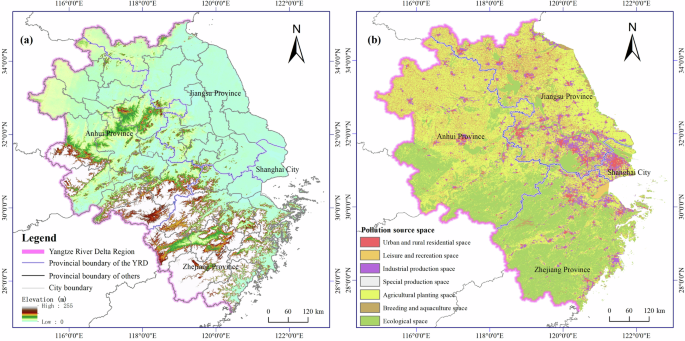
a Location; b Distribution of the pollution source space.

Full size image

From the perspective of interprovincial differences, industrial structure directly affects the types and distribution of pollutants in the YRD. Jiangsu actively develops secondary industries, accounting for 37.5% of the total industrial parks in the YRD. Industries such as metal manufacturing and textiles generate organic pollutants like chemical oxygen demand ((COD)) and volatile organic compounds ((VOC_S)). Anhui, an important agricultural base, accounts for 54.8% of livestock and poultry farming in the YRD. The use of nitrogen fertilizer and feed causes water eutrophication. Zhejiang’s 133 industrial parks primarily focus on pharmaceutical manufacturing and the new energy industry, generating less industrial solid waste and exhaust gas. However, large-scale aquaculture, accounting for 78.5% of seafood production, still leads to serious coastal water pollution. Shanghai’s urbanization rate has exceeded 88% due to its role as an international economic center, resulting in significant discharge of household waste and sewage from population agglomeration.

Technical process and methods

Concept and reclassification of pollution source space (PSS)

Environmental pollution sources are entities (e.g., device, place, and equipment) that release hazardous substances into the ecological system or have harmful effects on the environmental system. Currently, there is no universally established system or standardized classification for environmental pollution sources worldwide. Classification models used in the United States, Canada, and the European Union share similarities, with some based on spatial forms such as points, lines, and surfaces while others focus on social functions (U.S. Environmental Protection Agency, 2020; European Environment Agency, 2023; Government of Canada, 2023). In China, the State Council conducted the second national survey for the environmental pollution sources which identified industrial sources, agricultural sources, urban living sources, mobile sources, and centralized treatment sources as key targets. To further enhance our understanding of pollution sources beyond individual devices or equipment to encompass land space and consider multiple attributes including socio-economic factors, ecological environment conditions and geographical space relationships through land use patterns and associated pollution behaviors, we propose a new concept called pollution source space (PSS). Hence, we define the PSS as the land space that supports significant human production and living activities resulting in anthropogenic pollutants discharge leading to stress on the ecological environment system.

Based on homogeneity and similarity of pollution characteristics, we refer to standards such as the land use status classification (GB/T 21010-2007), the urban land and construction land use classification (GB 50137-2011), and the first national geographical survey of land use and land cover change (GDPJ 01-2013) to establish a classification system for PSSs (Xu et al., 2019), and then use artificial vectorization techniques combined with supervised classification to extract and map existing land use patches. We use the remote sensing tool (i.e., superSIAT-2.1 software) and random forest algorithm to extract land cover types, and combine spatial data like OpenStreetMap to generate pollution source samples. These land cover types are further refined into a detailed pollution source classification system. We also manually correct the classification results and overlay the data in ArcGIS software to create the final distribution map of the PSS.

Generally, at the regional or provincial scale, the PSSs can be broadly classified into three categories: urban space, agricultural space and ecological space, which are utilized for integration with national spatial planning. At the city or county scale, we further categorize them into eight types of PSSs (Fig. 1b): urban and rural residential space (URRS), leisure and reactional space (LRS), industrial and mining production space (IMPS), special production space, agricultural planting space, agricultural breeding space, general ecological space and ecological protection red line (EPRL). At a smaller village or grid scale, we can subdivide these eight types into more than 20 categories based on specific human activity types and land use attributes to align them precisely with other spatial planning measures (Table A1).

Here, we emphasize the definition, pattern extraction, and code setting of three types of the PSS:

1. (1)

   IMPS: it refers to spaces used for industrial production, product processing and manufacturing, as well as mining and quarrying areas and tailings storage areas. We initially use industrial land (land use classification code 0601) and mining area (code 0602) as the base map patches. These are combined with point of interest data for industrial points and mining sites to preliminarily identify the spatial agglomeration of industrial and mining areas. Further, we overlay various industrial parks, including national and provincial-level approved development zones, to delineate the IMPS.

2. (2)

   URRS: this primarily encompasses residential land (land use codes 071 and 072) in cities, towns, and villages. Due to the complexity of urban functions, such as commercial, educational, medical, and elder care services, it also includes public management and service land within cities and towns.

3. (3)

   EPRL: although ecological spaces involuntarily emit anthropogenic pollutants into the external environmental system, they can still inevitably produce trace amounts of such pollutants due to their ecological properties. We aim to retain EPRL as an environmental constraint indicator to control the extent of urban and agricultural spaces, and further delineate the subtypes of ecological space in accordance with national standards, such as EPRL policy and local ecosystem service function, to align with environmental control guidelines of varying intensities.

Hierarchical cluster analysis for pollution source structure

We employed the hierarchical cluster method to analyze the regional differences in the structure of pollution sources. Using SPSS software, we measured the sample distance of various pollution sources and automatically select the most suitable clustering threshold by Ward’s method. Effective clustering is indicated by a smaller sum of squared deviations within clusters and a larger sum between clusters (Xue, 2004). The sample distance is quantified by the squared Euclidean Distance, which is the sum of squared differences between the values of each variable in two samples (x,y). The formula (1) is as follows.

In the clustering process, we used the proportion of sulfur dioxide ((SO_2)) and (COD) emissions from different pollution sources in each county as clustering variables. We choose the agglomerative hierarchical clustering for the analysis, using the Euclidean distance as the distance metric to measure the similarities between the counties. It begins by treating each county as an individual cluster and progressively merging them based on their similarity until the desired number of clusters is achieved. We set the maximum number of clusters to five and the minimum to two. The optimal number of clusters was determined from the dendrogram, taking into account factors such as sample sizes, similarity levels, and the average emissions within each cluster. Ultimately, the optimal number of clusters was four for (SO_2) and 5 for (COD). After completing the clustering analysis, we exported the dendrogram results to Excel and created cluster distribution maps for different pollutants.

Environmental Stress Evaluation Model for PSS

We assume that anthropogenic pollution behavior does not autonomously occur in ecological spaces nor emit anthropogenic pollutants outwardly. Therefore, all calculation processes solely focus on urban and agricultural spaces characterized by intense human activities. The pollution stress intensity (PSI) of single factors reflects the level of water, soil, and air pollution generated by different PSSs from various perspectives. We employ the enhanced emission factor method to calculate the PSI of each PSS’s single factor pollutant discharge while determining the number of stress objects and stress coefficients associated with different pollution behaviors. This approach allows us to establish quantitative evaluation formula (2) effectively.

where (EM) is the PSI of each PSS, (EF) is the baseline stress coefficient for pollutants, (A) is the amount of stress objects, (delta) is the efficiency of pollution removal, (i) is the type of the PSS, (l) is the type of pollutant, (j) is the human pollution behavior, (k) is the type of stress object, and (z) is the pollution control measure. In practice, (EF) will be based on official environmental documents (e.g., Manual for Emission and Pollution Coefficients of Domestic Pollution Sources) and adjusted according to field survey data. (A) will depend on actual pollution behavior, referencing official statistics. (delta _z) will be derived from production processes, using standard values from production guidelines but adjusted for local industrial practices. For instance, to calculate the household waste generated by urban residential space (URS), we should determine the urban population (i.e., the amount of stress objects), per capita household waste generated (i.e., the stress coefficient), and household waste treatment rate (i.e., the efficiency of pollution removal) for a specific patch. The basic formula can evolve into other more detailed forms according to different pollution behaviors, such as fuel combustion, transportation, dust accumulation, livestock and poultry farming, and agricultural cultivation (Table A2).

We consult the national standards and the pollutant generation coefficient manuals for pollution sources across the four provinces of the YRD, compare pollution emission data from recent pollution declaration, environmental impact assessment reports and statistical yearbooks in the YRD, and make secondary corrections to the basic coefficient to determine the applicable stress coefficient specific to the YRD. Subsequently, we employ the symmetric weighting method (Formula 3) to ascertain weight value of the PSI of single factor, and obtain the integrated characteristic values (ICV) of solid waste, water pollutants and air pollutants for each PSS through weighted summation, which are used to reflect comprehensive environmental stress level.

where (omega) is the weight of pollutant, (barEM_l) is the average PSI of that pollutant generated by all PSSs, and (n) is the total amount of the PSSs. The degree of variation can reflect the impact or importance of different forms and types of pollutants on the ecological environment system. We could ensure that the relative error between the calculated PSI and environmental statistical data is controlled within 5%.

Structure optimization model of PSS based on multivariate linear programming

In December 2019, the Central Committee of the Communist Party of China issued the “Outline of the Development Plan for Regional Integration in the YRD,� highlighting the joint prevention and control of pollution in the YRD as a crucial aspect of regional integration. This outline serves as a guiding document for policy-making, covering a planning period up to 2025 and an outlook period extending to 2035. Hence, we utilize multivariate linear programming model to predict the spatial structure of urban, agricultural and ecological spaces for 2025 and 2035, and then estimate the PSI to elucidate the correlation between the PSSs and PSI.

We first clarified the concept of high-quality environmental development, defined as an integrated development model centered on sustainable human development, premised on green ecological development, and manifested through efficient governance (Fang et al., 2022). Target variable constraints are formulated under this strategic framework. Due to the urgent need for water environment management, strict control over water pollution is essential. As the focus of air environment governance shifts from traditional pollutants to emerging pollutants, such as ozone, it is crucial to ensure that emissions of traditional pollutants do not increase. We proposed that high-quality development objectives can be achieved through the optimization and regulation of national land use. When setting decision variables, it is essential that ecological space remains constant, urban space does not expand, and agricultural space is appropriately reduced. Since 2020, China’s territorial spatial planning has replaced previous land use and urban master plans, changing spatial classification models. We will calculate the average values for urban, agricultural, and ecological spaces from various planning documents to serve as constraints.

Based on the above constraints, we construct the multivariate linear programming model and propose four specific assumptions: firstly, decision variables (i.e., areas of the PSSs, (X_m,n,t)) are constrained by official spatial planning while simultaneously meeting constraints related to individual pollutants as well as those at provincial or regional levels within YRD (Table A3); secondly, target variables (i.e., the PSI, (Y_m,n,t)) are not strongly constrained by participating in model predictions but should ultimately meet indicator constraints outlined in important policy documents, such as the 14th Five Year Plan (Table A4); thirdly, all PSS in 2020 will be merged into urban, agricultural and ecological spaces, with emissions for each type calculated by province, and emission coefficients determined based on both emissions and spatial area; fourthly, the ecological space only serves as a total spatial constraint indicator due to no anthropogenic pollutant emissions. The objective function designed in Lingo software is as follows.

where (Y) is the PSI of each pollutant, (alpha) is the stress coefficient of each PSS, (X_1) is the area of urban space, (X_2) is the area of agricultural space, (X_3) is the area of ecological space, (m) is the type of regions, (n) is the type of pollutants, and (t) is the prediction year. The sum of (X_1), (X_2) and (X_3) should be the total land area of each province, and Y aims to achieve minimization and can refer to the range of regional pollution control, without any mandatory requirements.

Data sources

We utilize spatial data, including administrative division, land use, and EPRL, for reclassification of PSSs and basic spatial mapping (Table 1). Land use and EPRL are raster data, with a resolution of 30 m at county scale and 100 m at provincial scale. Vector data, such as administrative division, water system, and traffic network, are converted into raster data to ensure accuracy consistent with existing raster data. Subsequently, we employ environmental census data, along with economic and social statistical data, to calculate the PSI. Economic and social data are generally used to determine the quantity and location distribution of pollution sources. Additionally, since statistical data are often presented by administrative regions, we will rasterize this data into a 30-m grid and then match it with spatial data for calculation. For the missing spatial and statistical data, we conducted field surveys in Zhejiang and Jiangsu in 2021 and 2022, respectively. Through enterprise surveys, government interviews, and questionnaires, we manually mapped the PSSs that could not be identified through remote sensing, and supplemented the enterprise ledger data, which was used for verification and coefficient calibration.

All of the data were imported into ArcGIS software, where we assigned attributes to all raster units and used the raster calculator function to complete the calculation of the PSI. By consulting the pollution source coefficient manuals of China and comparing pollution declarations, environmental impact assessment reports, and pollution census of the YRD, we performed secondary adjustment to the national coefficient and optimize them to derive stress coefficients applicable to various provinces within the YRD. Additionally, local governments in China release annual pollution emission data at the county level (e.g., environmental statistical bulletins, environmental quality reports, et al.), covering pollutants such as (SO_2) and (COD). We aggregate the calculated source emissions at the county scale and compare them with official statistics, ensuring the standard error is within 5%, thereby meeting the accuracy requirements for spatial effect analysis.

Past clustering of environmental stress at the county level

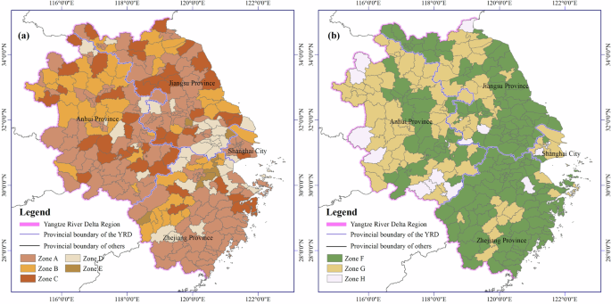
In 2010, the YRD emitted 3.15 million tons of (COD) and 2.37 million tons of (SO_2), which accounted for 25.45% and 10.82% of China’s total emissions, despite the region covering only 4% of the country’s land area. These pollutants have consistently been key targets for emission control by both central and YRD environmental authorities, reflecting their significance. Hence, we used hierarchical clustering to analyze the emission sources of (COD) and (SO_2) in 305 counties in the YRD, creating a cluster map with SPSS software. Then, we compared the clustering results with the county classifications from official planning like the YRD’s functional zoning plan, adjusting the clusters based on each county’s role in urban development, agriculture and ecological protection, as shown in Fig. 2.

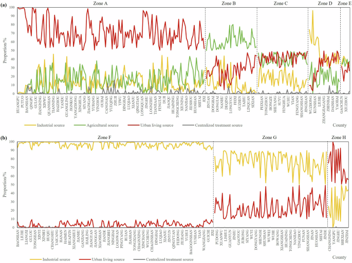
a COD structure; b SO₂ structure.

Full size image

Figure 2a presents the distribution of (COD) emission from industrial sources, agricultural sources, urban living sources, and centralized treatment sources, clustered into five zones to illustrate the spatial differentiation of water pollution sources at the county scale. Zone A encompasses 169 counties where urban living activities serve as the primary pollution source, contributing 71.43% of (COD) emissions, while industrial sources account for 12.43% and agricultural sources for 14.94%. Zone B consists of 46 counties predominantly influenced by agricultural activities, with livestock breeding and farming contributing 60.57% of (COD) emissions. Zone C comprises 45 counties relatively balanced contributions from urban living (41.68%) and agricultural activities (40.42%). Zone D includes 28 counties where both urban living (32.07%) and industrial sources (48.14%) are significant contributors to (COD) emissions, with nine counties showing industrial emissions exceeding 60%. Zone E represents 17 multi-source counties where industrial (36.84%), agricultural (35.75%), and urban living (26.87%) sources all contribute notably to emissions. Centralized treatment sources, such as sewage and waste treatment plants, have minimal impact on the clustering results due to their low emission proportions.

Figure 2b illustrates the cluster analysis of (SO_2) emission from industrial, urban living, and centralized treatment sources in the YRD, revealing three distinct zones. In 93.77% of counties, industrial emissions exceed 50%, with an average of 85.68% across the region, highlighting the significant impact of industrial exhaust on the atmosphere. Counties with industrial emissions over 90% are classified as Zone F, which includes 181 counties where industrial activities contribute 96.82% of (,SO_2) emissions. The remaining 104 counties, with industrial emissions between 50% and 90%, form Zone G, where industrial sources account for 77.28%, urban living sources for 22.71%, and centralized treatment sources for 1.13%. Zone H consists of 20 counties primarily influenced by urban living sources, where daily fuel combustion by residents contributes 71.57% of (SO_2) emissions, compared to 28.42% from industrial sources and 5.28% from centralized treatment.

Based on cluster analysis, we created a map showing the distribution of (COD) and (SO_2) emissions, as seen in Fig. 3. The map highlights a north-south divide in water pollution sources within the YRD. In the south, pollution mainly comes from urban living areas (Zones A, B, and E), while the north is dominated by agricultural sources (Zones B and C), particularly in major grain-producing regions. Shanghai and its surrounding areas have many industrial parks, classified as Zone D. For air pollution, there’s a strong east-west divide. The eastern coastal areas, including cities like Shanghai, Suzhou, and Hangzhou, saw rapid industrial growth in 2010, especially in sectors like biomedicine and manufacturing (Zones F and G). In contrast, western Zhejiang and Anhui focused more on tourism and services, leading to slower industrial development and less air pollution (Zone H).

a COD emission; b SO₂ emission.

Full size image

Current layout of environmental stress at the grid level

At the grid scale, we calculate the PSI for water and air pollution in the YRD in 2020 using 14 types of tertiary PSSs (Fig. 4). This analysis highlights the cumulative stress effects and spatial differences in pollution impacts on the environment. Water pollution stress exhibits a typical step effect in its spatial distribution across various sources. URS, rural residential space (RRS), and livestock breeding space (LPBS) have the highest emissions, with 203,600 tons, 193,200 tons, and 183,100 tons, respectively. Other contributors like cultural recreation space (CRS), pollution-intensive production space (PIPS), and grain growing space (GWS) emit between 20,000 and 50,000 tons, while the remaining areas contribute less than 10,000 tons. Sewage discharge is strongly linked to population density, especially in cities, increasing wastewater and sewage volumes. In LPBS, emissions depend on the scale of breeding activities, with lower emissions in Zhejiang and Shanghai due to restrictions on large-scale aquaculture. Non-point source pollution from soil erosion is also influenced by agricultural land distribution. Air pollution stress mainly comes from emissions in PIPS, general manufacturing production space (GMPS), and transportation space (TPS), contributing over four million tons collectively. Vehicle and machinery movement in TPS can spread pollution across other areas. Air pollution is closely related to energy use, with high-stress zones in areas like PIPS and TPS, while household energy consumption has a smaller impact. Therefore, air pollution control focuses on managing point sources and reducing emissions in industrial processes.

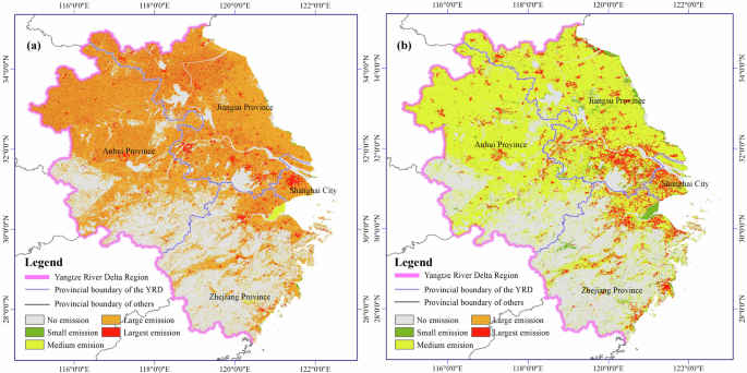
a Water pollutants emission, b Air pollutants emissions.

Full size image

Using the Jenks natural break classification method, along with pollution stress characteristics and treatment technologies, we classified the 14 PSSs into six pollution stress intervals: highest, high, medium, low, lowest, and no stress, based on ICV values (Fig. 5). The zero-pollution area (ICV = 0) covers 121,473.9 km², mainly in the southwest of Zhejiang and Anhui. Over 80% of this land is designated as a provincial EPRL, which enforces strict measures against pollutant discharge and prioritizes high-intensity ecological protection. The high-pollution area (ICV > 1) includes PIPS, mining space, LPBS, URS, and RRS, where urban and rural living sources, as well as industrial activities, combine to create high environmental stress. These areas make up only 14.65% of the land but have an average stress index of 1.41. This pattern is especially pronounced in rapidly urbanizing regions like Shanghai, Hangzhou, and Nanjing, where most of the population lives in urban areas and industrial parks. The low-pollution area (0 < ICV < 1) covers TPS, GMPS, aquaculture space, CRS, fruit and tea planting space, pollution treatment facilities, and natural recreation space. It accounts for 51.53% of the land, with an average stress index of 0.238, showing low spatial concentration and minimal pollution stress. Pollution from agriculture is closely linked to the distribution of grain production areas. Jiangsu and Anhui have significantly larger low-pollution areas (63.83% and 60.09%, respectively) due to their focus on high-quality farmland construction, compared to Zhejiang and Shanghai.

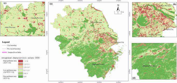
a Environmental stress distribution; b Typical area of high-pollution: Shanghai metropolitan area; c Typical area of low-pollution: Huaibei plain; d Typical area of zero-pollution: Ecological protection area.

Full size image

Future structure of environmental stress at the provincial level

The prediction of future scenarios primarily aims to address environmental structural regulation. Multivariate linear programming employed is an extension of linear regression. The equation must strictly follow the four principles outlined in the model design. Target variables are weak constraints, ensuring the minimization of pollutant discharge while aiming to achieve the goal of high-quality environmental development in the YRD by 2035. Decision variables are strong constraints, and their threshold values must be strictly set according to Tabel A4. All variables are non-negative, and the data sources for the variable values align with those used in other analyses, necessitating the testing of the regression model’s applicability before establishing target parameters. As shown in Table 2, there is a strong correlation between the decision variables and the target variable, with no collinearity detected. The model fits well, explaining nearly 50% of the variance in the target variables. Preliminary tests using 2020 data showed that (COD) emissions in Shanghai were estimated at 78,100 tons, compared to the actual 72,900 tons, resulting in a 7.18% error. Error margins for other pollutants were within 15%, confirming the accuracy of the predictions.

Then, we predict the spatial structure of PSSs across the entire YRD and its four provinces, estimating environmental stress for 2025 and 2035. Urban space in the YRD will remain stable at 46,700 km², while agricultural space is projected to decrease from 178,400 to 144,500 km² by 2025, before slightly increasing to 145,800 km² by 2035. In contrast, ecological space is expected to expand from 123,000 to 167,000 km² by 2025, stabilizing at around 165,700 km² by 2035. These trends align with national spatial planning for the YRD, with significant fluctuations mainly between 2020 and 2025. As shown in Table 3, changes in PSS structure across each province follow the same pattern as the overall YRD. Urban space remains largely unchanged, with a slight increase of just 0.93% in Shanghai, focusing mainly on internal optimization. Agricultural space shrinks notably. By 2035, agricultural space in Shanghai, Jiangsu, Zhejiang, and Anhui will decrease by 51.1%, 22.6%, 7.1%, and 17.5%, respectively. Despite these declines, farmland protection remains intact, ensuring major agricultural zones are preserved. Ecological space steadily expands, with increases of 26,000 km² in Shanghai, 33,600 km² in Jiangsu, 69,100 km² in Zhejiang, and 60,400 km² in Anhui. This growth underscores the importance of ecological protection in the high-quality development of the YRD.

Based on the quantitative changes in PSSs, we selected (COD), (NH_3-N), (SO_2) and (NO_x) as representative pollutants to predict pollution stress (Table 4). Compared to 2020, significant progress in controlling water pollution in the YRD is expected, with (COD) and (NH_3-N) emissions reduced by 34.7% and 38.7%, respectively, by 2035, aligning with both experimental constraints and local environmental planning requirements. For air pollution, emissions of (SO_2) and (NO_x) are projected to be controlled at 498,000 and 1,861,000 tons by 2035. While slightly higher than in 2020, these values remain within national standards. Over time, air pollution in the YRD has shifted from traditional to composite sources, with increasing levels of pollutants like (PM_2.5), (PM_10) and (O_3). Pollution stress changes across the four provinces follow similar trends as the entire YRD. The interaction between PSSs and PSI indicates that the sharp reduction in water pollutant emissions by 2035 is primarily driven by the rapid decrease in agricultural space. Meanwhile, air pollution remains largely influenced by domestic and industrial sources, with stable urban space leading to only minimal changes in air quality.

Each province shows strong compliance with water pollutant emissions, which remain well below experimental limits. Regarding water quality, Jiangsu stands out with the most significant reduction, as the province has many rivers and lakes, making water pollution control a key priority with notable success. In Anhui, as an agricultural powerhouse, water pollution control is closely linked to agricultural practices. The development of greener and more modern farming methods has significantly contributed to improving the province’s water environment. However, air pollutant emissions only meet national standards, not the weaker constraint conditions proposed during experimentation. In general, air pollutants show only small changes, indicating that the four provinces have effectively managed traditional air pollution, with a focus now shifting to the control of emerging pollutants. Additionally, the YRD has proposed integrated pollution management, with all four provinces adopting the same set of emissions standards. A cross-regional emissions trading system has been established to better address issues such as declining governance efficiency in border areas and collaborative environmental protection between upstream and downstream regions.

Causes of environmental stress evolution from the perspective of pollution sources

We quantified environmental stress across various scales—provincial, county, and grid levels, and found that environmental stress in the YRD exhibits both temporal and spatial heterogeneity, and the structure of pollution sources directly affects the type and intensity of environmental stress. The YRD stands out as China’s most representative and densely populated region, and it is also a leading area in achieving environmental sustainability. Other scholars have conducted research on the pollution pattern in the YRD or similar metropolitan areas worldwide, and discovered that the environmental stress exhibits dynamic spatial agglomeration and cross-border spillover characteristics (Becker and Henderson, 2000; Zhang et al., 2022). So, we explore the driving factors behind environmental stress from the perspective of human–environment interactions in economic geography. Classical theories like the Environmental Kuznets Curve have proved that economic growth and population development can positive or negative impacts on regional environment, with specific curve forms (e.g., inverted U-shaped, U-shaped, N-shaped, etc.) varying based on specific pollutant types and socio-economic development stages (Grossman and Krueger, 1991; Zaman et al., 2016; Xie et al., 2019). The EKC theory states that when a country’s GDP per person reaches a certain level, environmental quality starts to improve. In the YRD, the GDP per person in 2020 was 110,261.3 yuan, which is still below the inflection point of 173,251.8 yuan. This means that, for now, environmental quality has decreased from its peak but continues to worsen as the economy grows.

We also analyzed how humans and the environment interact in the YRD through OLS, SEM, and SLM models. Figure 6 illustrates that population size, industrialization level, urbanization level and fixed assets investment significantly contribute to increased environmental stress in the YRD, while foreign direct investment will negatively inhibit the stress. However, environmental problems are the outcome of the integrated actions within the human-land system. Besides regular economic and social activities, human beings can also modify the land cover type and ecosystem through land use changes (e.g., mode, intensity, structure, speed, etc.), and then feed back to the environment system. We, along with previous studies (Wang et al., 2021), have demonstrated that complex human interventions, such as land use transformation, affect regional environmental pollution levels and influence the stability of ecological systems by altering biodiversity, ecosystem service value, landscape patterns, etc.

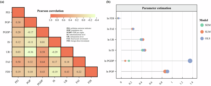
a Pearson correlation test; b Parameter estimation of the regression model.

Full size image

By applying economic geography methods, we captured spatial patterns of human-induced pollution, showing how human activities in urban, agricultural, and ecological spaces interact with pollution sources. At the provincial level, we analyzed urban, agricultural, and ecological spaces, exploring their relationship with pollutant emissions and defining pollution and land use constraints for macro-level structural regulation. At the county level, we examined urban living, industrial, agricultural, and centralized treatment sources, assessing their spatial distribution and agglomeration effects for meso-level characteristic regulation. At the grid scale, we focused on specific PSSs like URS, RRS, LPBS, etc., aiming for targeted micro-level targeted regulation. Examining the hidden environmental impacts of this multi-source transformation is crucial for tracing the full cycle of pollution generation, transport, and control.

Practical governance strategies for environmental stress control

The current governance system in the YRD mainly focuses on spatial functional evaluations. Most control units are classified into priority, ordinary, or delayed control, without addressing more specific regulatory issues (Wang et al., 2014; Chen et al., 2022). Environmental policies should be adjusted in a timely manner to align with changes in environmental stress patterns and local strategic needs. The “Outline of the YRD Regional Integration Development Plan� presents new requirements for high-quality environmental development by 2025 and 2035. We preliminarily predict the quantity changes in the PSS and the associated environmental stress, aiming to delineate future spatial patterns of pollution sources prior to environmental governance. By 2035, the URRS and LRS will be concentrated in the city center as distinct blocks while also dispersing to townships in point form. The IMPS will be centrally organized within unified industrial parks, strategically separated from the URRS to mitigate conflicts, and connected through the TPS in a linear arrangement. The focus will be on following China’s farmland protection policy, which means limiting changes in agricultural land use and stopping unnecessary expansions, except for essential GWS. Efforts will focus on enhancing the quality of agricultural land and standardizing the layout of the LPBS. Adhering to EPRL requirements, inefficient agricultural and degraded urban spaces may be restored to ecological status, promoting the establishment of a continuous ecological spatial pattern.

To develop more targeted environmental policies, we can combine earlier research on environmental functional zoning and propose environmental regulation index codes. This allows us to match adaptable governance schemes for each PSS through classification, hierarchical control, and code positioning. The environmental control types, levels, and pollution stress attributes of each PSS are clearly displayed in charts and can be easily retrieved by inputting specific attribute values. Under this system, regulation should align with macro-level zoning policies while adjusting intensity based on pollution characteristics and external constraints, selecting precise control measures like industrial access lists, monitoring standards, and pollution control processes to improve environmental control accuracy and effectiveness.

For PSS associated with industrial production and daily life, the primary objective is to prioritize clean production practices and implement stringent environmental control measures. In the case of PSS related to agricultural planting and livestock production, governance should focus on the spatial manifestations of environmental stress and their indirect effects on the ecosystem, necessitating moderate-intensity control measures. PSS centered on ecological protection must emphasize the balance between ecological integrity and pollution stress, adhering to state-mandated environmental control regulations by the state. Based on the policy principles outlined above, we can take the guidelines for the LPBS as an example. It is necessary to emphasize the management of both front-end emissions and end-of-pipe treatments while ensuring ecological function. It is also essential to optimize breeding area planning and enhance supporting pollution treatment initiatives to ensure standardized management. Furthermore, fostering connections between cultivation and breeding areas could facilitate the secondary utilization of irrigation and livestock wastewater, promoting a cost-effective approach to pollution management.

Limitations and prospects of the research

We analyze the evolution of environmental stress in the YRD across different periods to accurately identify the sources of environmental stress and target them for effective governance. Our current analysis separately analyzed the pollution source structure and the resulting environmental stress in 2010, 2020, and 2035. However, the research is conducted in phases of 10–15 years, with a relatively coarse temporal resolution, and we have not yet characterized the transfer pathways of environmental stress among different pollution sources. Moving forward, we will employ spatial explicit model and spatial exploratory analysis tools to elucidate the direction and mechanisms of pollution source transfer, thereby providing a clearer understanding of the spatial reconstruction of environmental stress. For instance, we can expand the land use transformation matrix to build an explicit transformation matrix for PSS, identifying the quantity, distribution, and flow of pollution sources.

In our scenario simulations, we mainly calculated changes in the quantity of PSSs and made a qualitative estimate of how the spatial patterns have evolved. In fact, human activities not only alter the structure of pollution sources but also affect their spatial patterns. Spatial changes under different scenarios will influence the formulation of environmental policies. For instance, point-source concentrated distributions and linear diffuse distributions will require different environmental governance measures. Going forward, we will use land use simulation models, e.g., flow-directed landscape unit segmentation, to visualize the spatiotemporal trends of PSSs under complex development policies, thereby informing the development of environmental governance plans. This improvement can address the threshold accuracy in the proposed multivariate linear programming, ensuring that the numerical limits of the PSSs are based not only on planning documents but also on the actual needs derived from socio-economic development projections.

Additionally, the current PSI calculations primarily focus on traditional pollutants, with some parameters derived through intermediate conversions, which could affect the accuracy of the results. Considering China’s dual-carbon target, future assessments will incorporate carbon dioxide and carbon monoxide as key characteristic pollutants, assigning appropriate weights to emphasize their significance in upcoming environmental regulation. In this way, we can reconstruct a new atmospheric environmental stress index that includes traditional air pollutants while also addressing the pressing issue of carbon emission control.

In conclusion, we reconstructed pollution sources and assessed environmental stress across various scales using spatial clustering, the enhanced emission factor method, and a multivariate linear programming model. Our findings reveal significant environmental stress at the county level in 2010. Urban living sources contribute to major water pollution in 55.4% of counties, while absolute industrial sources accounted for 59.3% of air pollution. By 2020, the YRD continued to face severe environmental threats. At the grid scale, pollution sources were categorized into high, low, and zero-stress, with average PSI of 1.41, 0.24, and 0, respectively. Guided by high-quality environmental development in 2035, emissions of (COD), (NH_3-N), (SO_2) and (NO_x) in the YRD are projected to controlled at 1,967,200, 99,200, 497,800, and 1,861,400 tons, respectively. To meet these targets, the urban, agricultural, and ecological spaces will be adjusted at 47,600, 145,800, and 165,700 km². Development policies affect human activities, pollution sources, and environmental stress. Based on this, a top-down environmental governance system can be established, implementing functional, structural, and usage controls at the macro, meso, and micro scales. Future research will focus on optimizing a comprehensive environmental stress indicator system, illustrating the specific transfer patterns of environmental stress over time and space, and identifying policy tools for different scenarios.