Interdecadal variability of terrestrial water storage since 2003
March 29, 2025
Abstract
Earth’s water cycle is changing due to anthropogenic forcing and internal variations in the climate system. These changes are leading to an intensification of the water cycle that manifests as more frequent and stronger droughts in some areas, and pluvials in others. The resulting impacts on terrestrial water storage can be crucial for water availability. However, current understanding is hampered by limitations in observations and models, and the variety of processes that influence terrestrial water storage across temporal scales. Here, we leverage the now two-decades long satellite record from the Gravity Recovery and Climate Experiment and subsequent Follow-On missions to investigate persistent trends in the presence of internal variability. We use cyclostationary empirical orthogonal function analysis to uncover statistical modes of variability that help explain a shift in decadal terrestrial water storage trends that occurred around 2012. The dominant statistical mode suggests an interdecadal periodicity that is also found in the precipitation record. The second leading mode is highly correlated with the Pacific Decadal Oscillation. Isolating these modes points to regions where the magnitude of the terrestrial water storage trend may flatten or reverse in coming decades due to internal climate variability and reduces uncertainty in multidecadal linear trends.
Introduction
Earth’s water cycle is changing due to anthropogenic forcing and internal variations in the climate system1,2. Thermodynamically, higher global temperatures are increasing evaporation and the atmosphere’s ability to store water3,4,5,6. Changing dynamical drivers are altering precipitation patterns and amplifying regional contrasts, especially between land and ocean7,8,9,10. Over the oceans, the dry subtropics are expected to get dryer, while relatively wet conditions are expected to continue in the tropics and extratropics (the ‘dry get dryer, wet get wetter’ paradigm)11. On land, however, the relationship is more ambiguous; climate-driven changes in the water cycle may be intensified by local dynamics (e.g., changes in moisture transport and/or mass convergence) and land-atmosphere interactions such as soil moisture and land-use changes1,12,13. Together, these factors are leading to an intensification of the water cycle that manifests as more frequent and stronger droughts in some areas, and pluvials (wetting events) in others across various timescales14,15,16,17,18.
Of direct concern for resource managers are the implications of water cycle changes on terrestrial water storage (TWS), which includes water in rivers, lakes, reservoirs, tree canopies, snow, soil and groundwater19. Understanding long-term TWS change is crucial for predicting future water availability, but characterizing these changes has been challenging due to limitations in observing systems20 shortcomings in model representation21,22,23,24 and human interventions (e.g., groundwater withdrawal)25,26,27. Moreover, internal climate variability, especially on timescales from seasonal to interdecadal, can temporarily dampen or amplify underlying secular TWS trends23,28,29,30,31,32.
The global satellite record of monthly mass change measurements from the Gravity Recovery and Climate Experiment (GRACE; 2002–2016) and subsequent Follow-On (GRACE-FO; 2018-present) missions enables tracking of TWS changes around the globe32,33. Observations from GRACE/GRACE-FO have informed how TWS changes across timescales, including seasonal variability34,35,36,37,38, interannual-to-interdecadal variability such as the El-Nino Southern Oscillation (ENSO) and the Pacific Decadal Oscillation (PDO)39,40,41,42, and longer-term variability suggesting secular trends25,37,43,44.
The GRACE/GRACE-FO satellite record, now over two decades in length and growing, enables us to better detect long-term trends in the presence of interannual and longer variability. Reference 31 used the then relatively short GRACE record (2002–2014) to attribute observed regional trends in TWS to climate variability, leaving open the question whether these trends would persist over the subsequent decade. With a longer record available, we now revisit the GRACE/GRACE-FO record to better understand which features can be linked to interdecadal climate variability and which persist throughout the multidecadal record and thus may be indicative of longer-term changes. The starting point of this study is a notable shift that occurred in the decadal regional trends of the GRACE TWS record that continued through the initial phase of the GRACE-FO mission.
Results
Many regions around the world experienced a shift in linear TWS trends between the first half (2003–2013; Fig. 1a) and second half (2013–2023; Fig. 1b) of the GRACE/GRACE-FO record. Over ice-free land (see Materials and Methods), the area-weighted spatial Pearson correlation coefficient (�) between the regional trend maps of the first and second half of the record was � = 0.49. (Fig. 1c). 28.0% of locations (grid cells) underwent a significant reversal in trend direction from the first half of the record to the second half (Fig. 1d; see Materials and Methods Eq. 2), split equally between locations that switched from drying to wetting conditions (13.6%) and wetting to drying (14.3%). The strength of dry conditions changed in 15.7% of locations, and the strength of wet conditions changed in 8.2%, resulting in a significant shift of TWS trends in a total of 51.9% of ice-free land between 60° S/N. The most pronounced trend reversal occurred in Southern Africa, where a wetting trend of 2.4 ± 0.5 cm/yr during the first half of the record switched to a drying trend of −0.9 ± 0.4 cm/yr during the second half (Supplementary Fig. 1). The strongest reversal from dry (−1.2 ± 0.6 cm/yr) to wet conditions (1.0 ± 0.6 cm/yr) occurred in the north of Western Australia.
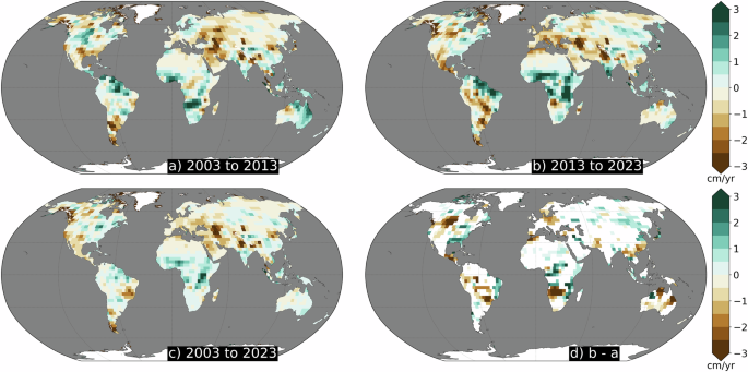
a January, 2003 to June, 2013; (b) July, 2013 to December, 2023; and (c) January, 2003 to December, 2023, and (d) the trend difference at locations where the sign is different between the first and second half of the record, such that positive (green) numbers indicate a reversal from drying to wetting, negative (brown) from wetting to drying, and white do not experience significant changes. Ice-covered regions are excluded.
In 45.9% of locations, the trends observed during the first half of the record differ significantly from those computed over the full record. The sign of the trend changed in 18.9% of total locations, with 15.4% undergoing a change in dry conditions, and the remaining 11.6% experiencing a change in wet conditions. The second half of the record underwent similar changes: overall 45.0% of trends shifted significantly, with 14.0% of locations reversing sign, 18.2% experiencing changes in dry conditions, and 12.8% undergoing a change in wet conditions.
Previous studies (see Introduction) have highlighted the influence of ENSO and the PDO on changes in TWS. Focusing on the longer timescales associated with the PDO, differences in the trend maps can be partly linked to the PDO (Supplementary Fig. 2a). During 2003–2013, the magnitude of the global mean correlation coefficient between the PDO and TWS was � = 0.36 with a 1-σ spatial variation of 0.20. During 2013 to 2023, it increased to � = 0.43 with a spatial variation of 0.24. However, locations that experienced trend reversals were poorly correlated with the PDO ( | � | = 0.16 ± 0.11) during the full record and modestly correlated at locations that experienced significant drying (|�|=0.29 ± 0.11) and wetting trends (|�|=0.33 ± 0.12). While not definitive, this simple correlation analysis indicates that the shift in trends observed during the first and second halves of the GRACE/GRACE-FO record are not fully represented by the PDO, and that other modes of variability or anthropogenic processes are at work.
To more robustly identify the common modes of variability in TWS, we performed a cyclostationary empirical-orthogonal function (CSEOF) decomposition on the gap-filled GRACE/GRACE-FO record (see Materials and Methods). The CSEOF method decomposes space-time data into a series of modes comprised of a spatial component (loading vector; LV) that varies with a ‘nested’ periodicity and a corresponding temporal component here referred to as the principal component time series (PCTS)45. Hereafter, the term ‘mode’ to refer exclusively to these statistical CSEOF modes, with explicit notations where additional analysis relates them to physical plausible internal climate modes.
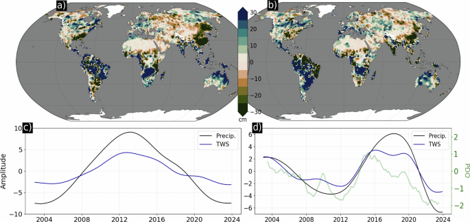
The first nonseasonal loading vector (LV; Fig. 2a) and its associated PCTS (Fig. 2c) contains 13.2% of the variance and indicates a reversal of TWS in November 2012. We find a spatial correlation coefficient of � = 0.38 between the loading vector and the TWS rates during the first half of the GRACE/GRACE-FO record, and � = −0.58 during the second half. This decreased to � = 0.23 over the full record, showing that variability in this mode impacted linear trends particularly strongly during 2013 to 2023. The most pronounced effects occurred in British Columbia, where TWS oscillated from a low of −9.5 cm to a high of 12.9 cm, for a peak-to-peak amplitude change of 22.5 cm. Though containing only one wavelength, the phasing hints at a multidecadal periodicity.
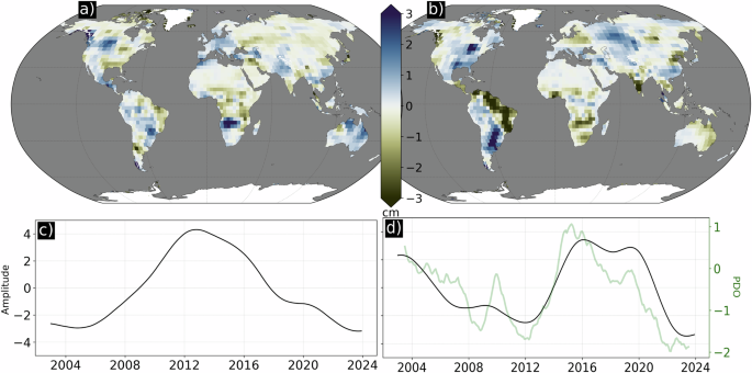
a Mode 2 loading vector containing 13.2% of the variance; (b) mode 3 loading vector containing 9.7% of the variance; (c) mode 2 principal component time series indicating a TWS shift in November 2012; and (d) mode 3 principal component time series (black) and Pacific Decadal Oscillation (PDO) index (green).
The following (second nonseasonal) CSEOF mode 3 contains 9.7% of the variance and is strongly correlated with the PDO (� = 0.81; Fig. 2b, d). We find a spatial correlation coefficient of −0.38 between the loading vector and the TWS rates during the first half of the GRACE/GRACE-FO record, and −0.30 during the second half. Over the full record, � decreased to 0.04. That is, this mode contributes to the trends seen in the first and second halves of the records, but not to trends over the full record. The most prominent feature is the dipole in South America (Fig. 2b): when the north and eastern coastline of the continent, from Colombia to Rio De Janeiro (including ~1000 km inland), is experiencing strong negative (dry) conditions, a wide north/south aligned swath stretching from the center of Brazil to Buenos Aires, Argentina experiences strong positive (wet) conditions. Specifically, the northeast (central/south) region oscillates by 27.3 cm (19.0 cm) and is strongly correlated with the PDO index (� = −0.80; 0.82).
Together, the two modes together explain 17.8% of the variance in TWS spatially averaged over ice-free land, with a one standard deviation range of 15.1% (Fig. 3a; see Materials and Methods). Linear trends explain 43.0% of the variance with a 31.5% standard deviation. At locations that experienced a trend reversal significantly different than 0, the modes explain 25.2 ± 16.2% of the variance. At locations with a persistent drying trend, 10.3 ± 13.5% of the variance is explained by the modes, while 16.2 ± 15.7% is explained at locations with a persistent wetting trend. Comparing pixel wise the variance explained by the combined modes vs that explained by a linear trend, we find that the combined modes explain slightly less variance than the linear trends (45.2% vs 54.8%; Fig. 3b). However, where the statistical modes are more important, they explain on average 25.7% of the variance, whereas where the trend is more important, they explain on average 46.2% of the variance.
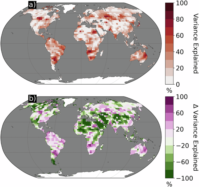
a Percent variance explained by the combined CSEOF modes 2 and 3. b The difference in variance explained by the combined modes of variability and linear trend. Positive (negative) percentages show where the modes of variability explained more (less) of the variance than linear trends during 2003 to 2023.
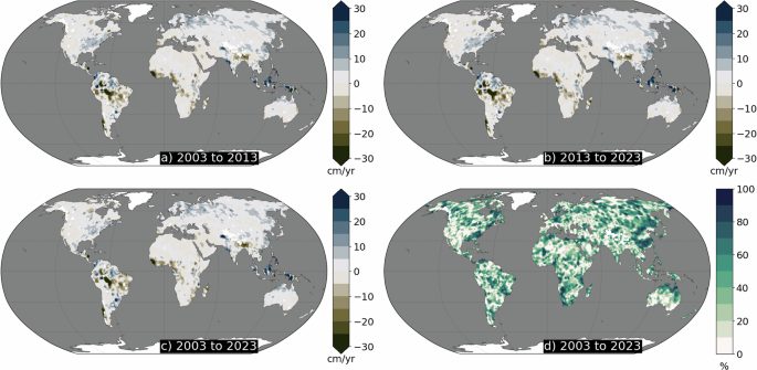
After removing the reconstructed modes of variability from the TWS time series, the regional trends maps across the three temporal intervals are indistinguishable (Fig. 4a–c). The spatial correlation between the first and second halves of the record increases from � = 0.49 prior to mode removal to � = 0.97 after removal. Additionally, after mode removal the signature of the PDO is substantially reduced (Supplementary Fig. 2). There are no locations that undergo trend shifts significantly different than 0 from one decade to the next. Only 4.2% of trends remained significantly different in the first decade relative to the full record, and only 0.3% were significantly different in the second decade relative to the full record. Globally averaged, removing the modes of variability reduces the uncertainty in the linear rates by 6.3 ± 12.0% during 2003 to 2013, 13.2 ± 21.4% during 2013 to 2023, and 26.3 ± 18.2% during 2003 to 2023, with the range representing one standard deviation of spatial variability (Fig. 4d). In the first half of the record, removing the modes increases the uncertainty of the trends in 26.5% of grid-cell locations; in the second half, mode removal increases trend uncertainty in 17.4% of locations. These locations are predominantly (71.1%) located in ‘Dry’, ‘Polar’, or ‘Snow’ climates46 characterized by stable trends from the first to second half of the record and low uncertainty (< = 0.1 cm/yr). Uncertainty did not increase after removing the modes from the full multidecadal record.
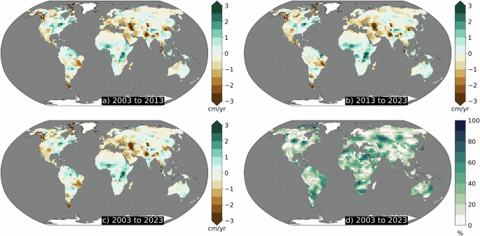
a 2003–2013, (b) 2013–2023 and (c) 2003–2023. d Percent reduction in trend uncertainty after removing combined CSEOF modes 2 and 3.
As precipitation is an important contributor to TWS, we analyzed cumulative precipitation anomalies using gridded observations from the Global Precipitation Climatology Center (GPCC; see Materials and Methods). The interdecadal variability observed in TWS is also found in precipitation, with a similar shift in trends computed over 2003–2013 and those computed over 2013–2023 (Fig. 5). Overall, 66.2% of precipitations trends over ice-free land between 60° S/N in 66.2% underwent significant shifts, with 10.6% of locations showing a significant change in dry conditions and 14.7% experiencing a significant change in wet conditions. The 40.9% of locations where trends in precipitation reversed sign largely align with those in TWS (c.f. Fig. 5c, d), especially in southern Africa, northwestern Australia, and the southeastern U.S. Notable exceptions, for example in southern China, suggest areas where surface and groundwater use may impact TWS and precipitation differently47.
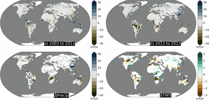
a January 2003 to June 2013 and (b) July 2013 to December 2023. c The trend difference at locations where the sign is different between the first and second half of the record, such that positive (blue) numbers indicate a reversal from drying to wetting, and negative (brown) from wetting to drying and insignificant trend differences are white. d As in (c), except for TWS (reproduction of Fig. 1d).
As with TWS, we identified dominant statistical modes of variability in precipitation through CSEOF decomposition (Fig. 6). The first mode (Fig. 6a) contains 45.3% of the variance in the precipitation timeseries, and its loading vector correlates strongly with the trend map in both the first (� = 0.61) and second (� = −0.68) decades of the record. The associated PCTS (Fig. 6c) shows that this is the same as TWS mode 2. In the next mode, we find interdecadal variability that again closely matches the PDO (Fig. 6d; � = 0.73), though the loading vectors are not as clearly implicated in the trends over the two decades of the record (� = −0.15, � = −0.17, respectively).
a mode 1 loading vector containing 45.3% of the variance; (b) mode 2 loading vector containing 17.8% of the variance; (c) mode 1 principal component time series of precipitation and TWS; and (d) mode 2 principal component time series of precipitation and TWS overlaid on the Pacific Decadal Oscillation (PDO) index (green). Note that TWS PCTS are those shown in Fig. 2.
We therefore removed only the first mode of variability from the original cumulative precipitation timeseries. As with TWS, this eliminates the differences between trend maps computed over the first and second decades of the record (Fig. 7). The correlation between trends computed over 2003 to 2013 with those computed from 2013 to 2023 increased from � = 0.19 to � = 0.99. There were no significant trend shifts from one decade to the next. The percentage of significant trend differences dropped from 54.6% to 11.1% when comparing the first decade to the full record and from 48.5% to 13.6% when comparing the second decade to the full record. The uncertainty on the trend (2003−2023) was reduced by 34.1 + /−25.5% (Fig. 7d).
a 2003−2013, (b) 2013−2023 and (c) 2003−2023. d Percent reduction in trend uncertainty after removing CSEOF mode 1.
Discussion
This study identifies a significant shift in TWS anomalies within the GRACE/GRACE-FO record (Fig. 1) and uncovers statistical modes of variability that help explain this shift (Fig. 2). Figure 3 highlights regions where interdecadal variability represented by these modes accounts for more of the changes in TWS than a linear trend model (e.g., Northern South America, Southern Africa, Australia), and regions where linear trends are dominant (e.g., the Southwestern U.S., Northern Africa, and the Arabian Peninsula). By removing these modes from TWS (Fig. 4), we effectively minimize the influence of interdecadal variability, reducing uncertainty of the ~21-year linear trend captured in GRACE/GRACE-FO. To gain physical insight into TWS trends, we conducted a parallel investigation of cumulative global precipitation anomalies, finding a similar trend shift between the first and second decades of the 21st century (Fig. 5) and modes that largely capture this shift (Fig. 6). As with TWS, removing the mode minimizes the influence of interdecadal variability (Fig. 7).
Taken together, these findings show where interdecadal variability likely caused trends computed over the first and second half of the record to deviate from those observed over the full record. This suggests that interdecadal variability can significantly alter water availability, such that the available ~21-year trend is not on its own a suitable measure for characterizing changes through time in over 50% of ice-free land. This is particularly evident in regions that are strongly impacted by interdecadal variability like southern Africa (Supplementary Fig 1), which has strong trends in opposite directions that cancel out over the full record. We also identify many regions (48.1% for TWS, 33.8% for precipitation) where linear trends adequately characterized TWS changes on decadal and longer timescales. Additionally, removing the estimated interdecadal variability from the full 21-year record has negligible impact on the regional trends (cf. Figs. 1c, 4c; Supplementary Fig. 3).
However, 21 years is still a relatively short record length for robustly identifying interdecadal variability. We can shed more light on this by investigating historical precipitation variability, extending our analysis by applying CSEOF analysis to the precipitation record from 1960 to present (Fig. 8). The 3rd mode, explaining 7.2% of the variance, contains the trend shift identified in the shorter records of TWS and precipitation (Fig. 8c). The parabolic feature within the PCTS now contains a second wavelength that hints at a ~ 30-year periodic variability in the water cycle. Additionally, this second wavelength undermines the possibility that the feature is linked to long-term acceleration, which would also manifest as a parabola-shaped PCTS (since the linear trend was removed prior to the decomposition). Mode 6, explaining 2.3% of the variance, corresponds to the decadal variability mode computed over 2003–2023 during the shared time period (Fig. 8d). After ~1990, the PCTS resembles the lower frequency PDO index. However prior to 1990, the mode is not correlated with the PDO but rather is noticeably out of phase.
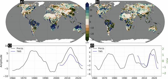
a mode 3 loading vector containing 7.2% of the variance; (b) mode 6 loading vector containing 2.1% of the variance; (c) mode 3 principal component time series of precipitation and TWS; and (d) mode 6 principal component time series of precipitation and TWS overlaid on the Pacific Decadal Oscillation (PDO) index (green). Note that TWS PCTS are those shown in Fig. 2.
This suggests sources of interdecadal variability that complicate the PDO influence on the CSEOF mode, warranting further investigation with more targeted analysis, such as CSEOF decomposition with longer nested periods.
Indeed, to fully understand interdecadal variability and long-term trends, particularly in the context of ongoing climate change, a more robust physically based diagnosis of the water cycle is essential. Recent research18 has addressed processes on seasonal to interannual timescales, but a similar understanding on longer timescales remains elusive. There are substantial challenges to investigate past interdecadal variability given the paucity of long-term, large-scale records, though there is evidence for increasing precipitation variability48 and bounds from model experiments on expected TWS variability29. Additionally, there are considerable obstacles in attributing trends in TWS to either internal variability or forced change given they can be strongly driven by anthropogenic surface and ground water use which are poorly constrained in, or altogether absent from, models25,49,50,51. In particular, areas with differing TWS and precipitation shifts (Fig. 5c, d) could yield insight into TWS changes driven directly by human water needs rather than interdecadal variability or long-term trends44. While trends in precipitation are not directly attributable to anthropogenic water use, they are linked to broader anthropogenic influence that is likely to change not only the mean state, but the nature of internal variability29,52. The period from 2003 to 2023 also contains several extreme ENSO events and longer precipitation extremes17,49 which may have contributed to making the GRACE/GRACE-FO record historically atypical. Further work should explore this and other potential nonlinear interactions, potentially using large ensemble model experiments52,53 to optimally account for the role of internal variability in observed trend shifts.
Nevertheless, our findings show that interdecadal variability can alter TWS such that decadal trends exhibit significant shifts, including changes in sign from one decade to the next. In the two decades examined here, about half of ice-free land is found to deviate substantially from a 21-year trend, reflecting the dynamic nature of TWS and precipitation variability, while the other half experiences a consistent multidecadal linear-trend that may persist in the future. To support effective water resource management, continued global gravity measurements (e.g., the upcoming GRACE-Continuity mission) and new high-resolution observations (e.g., from the Surface Water and Ocean Topography mission) are crucial for enhancing water resilience both now and in the future.
Materials and Methods
Data
We used monthly gridded estimates of equivalent water thickness based on retrievals from GRACE/GRACE-FO. Specifically, we used the monthly mascon solutions with coastal resolution improvement from release 061 version 03 generated by the NASA Jet Propulsion laboratory54,55. These solutions are resampled from the standard spatial resolution of 3 degrees (~300,000 km2) to a regular grid of 0.5° spatial resolution. While GRACE/GRACE-FO provides measurements over the ocean, only data over land is used here. We therefore refer to the liquid water equivalent values (which are anomalies relative to the mean gravity field) as simply TWS. We filled gaps within and between the GRACE/GRACE-FO record using a technique similar to that described in ref. 56. for the reconstruction of TWS from 1970 to 2020.
The reconstruction – and by extension gap-filling – technique used here relies on cyclostationary empirical orthogonal functions (CSEOFs). Empirical orthogonal function (EOF) analysis is a common technique for identifying modes of variability in climate studies. EOFs are limited in that each mode consists of a single spatial pattern and associated principal component time series that shows the change in amplitude of this spatial pattern through time. In contrast, CSEOFs have an additional structural periodicity (called the nested period), which allows the spatial pattern to vary within each mode45,57. The nested period is chosen based on some knowledge of the datasets being analyzed and the signals that are present within that data set. For example, if investigating the annual cycle in a monthly data set, a 12-month nested period would be selected, and each subsequent CSEOF mode would have one loading vector (LV) containing 12 maps (one for each month), and a principal component time series (PCTS) representing the amplitude modulation of this pattern through time.
For the analysis conducted here, a 2-year nested period is used to target variability associated with ENSO, which has been used effectively to understand climate and TWS variability28,58. Using the window provided by the nested period, any gap of less than 2-years can be filled by projecting the individual monthly maps of the LV onto data where available. In other words, when filling the gap between GRACE and GRACE-FO, actual GRACE data supports the projection of the LV on the front side of the window, while GRACE-FO supports the projection on the back side. This produces a representation of the PCTS at the midpoint of the window, and the LV can be moved one month at a time to fill the entire gap. The final step is to recombine the reconstructed and gap-filled PCTS with the associated LV to reform a TWS dataset from 2002 to present that is free of gaps. The results of the gap-filling relative to the underlying GRACE/GRACE-FO datasets are shown in Supplementary Figs. 4–6. The average annual cycle is preserved through the gap-filling process (Supplementary Fig. 4), and there are negligible differences in the TWS rates from 2002 to 2023 between the original data and gap-filled datasets (Supplementary Fig. 5).
To investigate the relationship between precipitation and TWS on annual timescales, we also use precipitation measurements from the GPCC at monthly resolution with 1.0° spatial resolution59. Cumulative precipitation is computed by at each timestep (month) as the sum of all previous timesteps.
Trend analysis and uncertainty quantification
Linear trends (β) are computed pixel wise via ordinary least squares that accounts for seasonal cycle (c1-4):
We characterize uncertainty as:
where t is the t-statistic corresponding to the 95% confidence interval and n-2 degrees of freedom, the standard error of the trend ((S(SE_beta ),=,sqrtmathrmvar(beta )), and ACF1 is the lag-1 autocorrelation. Trends shifts from the first to the second half of the record are deemed insignificant if the uncertainty adjusted rate interval of the first half overlaps with the uncertainty adjusted rate interval of the second half. Similarly, comparisons between one half of the record and the full record are only considered significant when the uncertainty adjusted rate intervals do not overlap. Additionally, locations with trend uncertainties that contain 0 in both comparisons (half vs half, or half vs full) are considered insignificant.
Percent variance explained by the combined modes is calculated as:
where TWS is the original TWS time series at location x and subscript REC is TWS reconstructed from CSEOF modes 2 and 3.
The strongest trend reversal regions are identified by first isolating pixels that experience a significant trend in both halves of the record of different sign. We then isolate regions by selecting contiguous groups of ten pixels or more with same direction reversals (from wetting to drying or vice versa). Next, we again cull regions with insignificant trends in either half of the record. Finally, we manually inspect the regions to ensure that they are greater than ~1 masocn (300 km) in size. For the modal analysis, we only consider pixels lower (higher) than the 10th (90th) percentile. We mask ice covered areas by rasterizing the mask available from Natural Earth (https://www.naturalearthdata.com/downloads/110m-physical-vectors/110m-glaciated-areas/). Spatial averages are weighted by the cosine of the latitude. We additionally consider only pixels between 60°S to 60°N when calculating percents.
CSEOF analysis
We apply the CSEOF analysis to pixel-wise linearly detrended gap-filled data. The annual cycle in GPCC was removed prior to decomposition but retained in TWS. Loading vectors (Figs. 2a, b, 6a, b, 8a, b) are averaged over the 2-year nested period as justified above. We note that applying EOF rather CSEOF analysis does not impact our findings. For example, the TWS CSEOF Mode 2 loading vector (PCTS) has a Pearson correlation coefficient of � = 0.93 (0.96) with EOF Mode 2.
Data availability
GRACE/GRACE-FO data are available from the NASA Physical Oceanography Distributed Active Archive Center at https://podaac.jpl.nasa.gov/dataset/TELLUS_GRAC-GRFO_MASCON_CRI_GRID_RL06.1_V3. GPCC precipitation data are available from the the NOAA Physical Sciences Lab at: https://www.psl.noaa.gov/data/gridded/data.gpcc.html. The glacier mask is available from Natural Earth at: https://www.naturalearthdata.com/downloads/110m-physical-vectors/110m-glaciated-areas/).
References
-
Herrera, D. A. et al. Observed changes in hydroclimate attributed to human forcing. PLOS Clim. 2, e0000303 (2023).
-
Douville, H. et al. Water Cycle Changes. In Climate Change 2021: The Physical Science Basis. Contribution of Working Group I to the Sixth Assessment Report of the Intergovernmental Panel on Climate Change [Masson-Delmotte, V., P. Zhai, A. Pirani, S. L. Connors, C. Péan, S. Berger, N. Caud, Y. Chen, L. Goldfarb, M. I. Gomis, M. Huang, K. Leitzell, E. Lonnoy, J. B. R. Matthews, T. K. Maycock, T. Waterfield, O. Yelekçi, R. Yu, and B. Zhou (eds)]. Cambridge University Press, Cambridge, United Kingdom and New York, NY, USA, 1055–1210, https://doi.org/10.1017/9781009157896.010.(2021).
-
Allan, R. P. et al. Physically consistent responses of the global atmospheric hydrological cycle in models and observations. Surv. Geophys. 35, 533–552 (2014).
-
Forster, P. et al. The Earth’s Energy Budget, Climate Feedbacks, and Climate Sensitivity. In Climate Change 2021: The Physical Science Basis. Contribution of Working Group I to the Sixth Assessment Report of the Intergovernmental Panel on Climate Change [Masson-Delmotte, V., P. Zhai, A. Pirani, S. L. Connors, C. Péan, S. Berger, N. Caud, Y. Chen, L. Goldfarb, M. I. Gomis, M. Huang, K. Leitzell, E. Lonnoy, J. B. R. Matthews, T. K. Maycock, T. Waterfield, O. Yelekçi, R. Yu, and B. Zhou (eds)]. Cambridge University Press, Cambridge, United Kingdom and New York, NY, USA, 923–1054, https://doi.org/10.1017/9781009157896.009.(2021).
-
Held, I. M. & Soden, B. J. Robust responses of the hydrological cycle to global warming. J. Clim. 19, 5686–5699 (2006).
-
Zhang, Y. et al. Multi-decadal trends in global terrestrial evapotranspiration and its components. Sci. Rep. 6, 19124 (2016).
-
Liu, C. & Allan, R. P. Observed and simulated precipitation responses in wet and dry regions 1850–2100. Environ. Res. Lett. 8, 034002 (2013).
-
Polson, D. & Hegerl, G. C. Strengthening contrast between precipitation in tropical wet and dry regions. Geophys. Res. Lett. 44, 365–373 (2017).
-
Roderick, M. L., Sun, F., Lim, W. H. & Farquhar, G. D. A general framework for understanding the response of the water cycle to global warming over land and ocean. Hydrol. Earth Syst. Sci. 18, 1575–1589 (2014).
-
Schurer, A. P., Ballinger, A. P., Friedman, A. R. & Hegerl, G. C. Human influence strengthens the contrast between tropical wet and dry regions. Environ. Res. Lett. 15, 104026 (2020).
-
Byrne, M. P. & O’Gorman, P. A. The Response of Precipitation Minus Evapotranspiration to Climate Warming: Why the “Wet-Get-Wetter, Dry-Get-Drier� Scaling Does Not Hold over Land*. J. Clim. 28, 8078–8092 (2015).
-
Seneviratne, S. I. et al. Investigating soil moisture–climate interactions in a changing climate: A review. Earth-Sci. Rev. 99, 125–161 (2010).
-
Yeh, S.-W., Song, S.-Y., Allan, R. P., An, S.-I. & Shin, J. Contrasting response of hydrological cycle over land and ocean to a changing CO2 pathway. npj Clim. Atmos. Sci. 4, 53 (2021).
-
Ficklin, D. L., Null, S. E., Abatzoglou, J. T., Novick, K. A. & Myers, D. T. Hydrological intensification will increase the complexity of water resource management. Earth’s Future 10, e2021EF002487 (2022).
-
Huntington, T. G. Evidence for intensification of the global water cycle: Review and synthesis. J. Hydrol. ((Amst.)) 319, 83–95 (2006).
-
Huntington, T. G., Weiskel, P. K., Wolock, D. M. & McCabe, G. J. A new indicator framework for quantifying the intensity of the terrestrial water cycle. J. Hydrol. ((Amst.)) 559, 361–372 (2018).
-
Rodell, M. & Li, B. Changing intensity of hydroclimatic extreme events revealed by GRACE and GRACE-FO. Nat. Water. 1, 241–248 (2023).
-
Swain, D. L. et al. Hydroclimate volatility on a warming earth. Nat. Rev. Earth Environ. 6, 35–50 (2025).
-
Oki, T. & Kanae, S. Global hydrological cycles and world water resources. Science 313, 1068–1072 (2006).
-
Greve, P. et al. Global assessment of trends in wetting and drying over land. Nat. Geosci. 7, 716–721 (2014).
-
Humphrey, V., Rodell, M. & Eicker, A. Using Satellite-Based Terrestrial Water Storage Data: A Review. Surv. Geophys. 44, 1489–1517 (2023).
-
Jensen, L., Eicker, A., Dobslaw, H., Stacke, T. & Humphrey, V. Long-term wetting and drying trends in land water storage derived from GRACE and CMIP5 models. J. Geophys. Res. Atmos. 124, 9808–9823 (2019).
-
Kumar, S., Allan, R. P., Zwiers, F., Lawrence, D. M. & Dirmeyer, P. A. Revisiting trends in wetness and dryness in the presence of internal climate variability and water limitations over land. Geophys. Res. Lett. 42, 10,867–10,875 (2015).
-
Scanlon, B. R. et al. Global models underestimate large decadal declining and rising water storage trends relative to GRACE satellite data. Proc. Natl. Acad. Sci. USA 115, E1080–E1089 (2018).
-
Rodell, M. et al. Emerging trends in global freshwater availability. Nature 557, 651–659 (2018).
-
Scanlon, B. R. et al. Global water resources and the role of groundwater in a resilient water future. Nat. Rev. Earth Environ. 4, 87–101 (2023).
-
Vishwakarma, B. D., Bates, P., Sneeuw, N., Westaway, R. M. & Bamber, J. L. Re-assessing global water storage trends from GRACE time series. Environ. Res. Lett. 16, 034005 (2021).
-
Cheon, S.-H., Hamlington, B. D., Reager, J. T. & Chandanpurkar, H. A. Identifying ENSO-related interannual and decadal variability on terrestrial water storage. Sci. Rep. 11, 13595 (2021).
-
Fasullo, J. T., Lawrence, D. M. & Swenson, S. C. Are GRACE-era Terrestrial Water Trends Driven by Anthropogenic Climate Change? Adv. Meteorol. 2016, 1–9 (2016).
-
Hamlington, B. D. et al. Origin of interannual variability in global mean sea level. Proc. Natl. Acad. Sci. USA 117, 13983–13990 (2020).
-
Reager, J. T. et al. A decade of sea level rise slowed by climate-driven hydrology. Science 351, 699–703 (2016).
-
Rodell, M. & Reager, J. T. Water cycle science enabled by the GRACE and GRACE-FO satellite missions. Nat. Water 1, 47–59 (2023).
-
Tapley, B. D. et al. Contributions of GRACE to understanding climate change. Nat. Clim. Chang. 9, 358–369 (2019).
-
Hamlington, B. D., Reager, J. T., Chandanpurkar, H. & Kim, K. Y. Amplitude modulation of seasonal variability in terrestrial water storage. Geophys. Res. Lett. 46, 4404–4412 (2019a).
-
Humphrey, V., Gudmundsson, L. & Seneviratne, S. I. Assessing Global Water Storage Variability from GRACE: Trends, Seasonal Cycle, Subseasonal Anomalies and Extremes. Surv. Geophys. 37, 357–395 (2016).
-
Schmidt, R. et al. Hydrological Signals Observed by the GRACE Satellites. Surv. Geophys. 29, 319–334 (2008).
-
Swenson, S. & Wahr, J. Monitoring the water balance of Lake Victoria, East Africa, from space. J. Hydrol. ((Amst.)) 370, 163–176 (2009).
-
Wahr, J., Swenson, S., Zlotnicki, V. & Velicogna, I. Time-variable gravity from GRACE: First results. Geophys. Res. Lett. 31, L11501 (2004).
-
Boening, C., Willis, J. K., Landerer, F. W., Nerem, R. S. & Fasullo, J. The 2011 La Niña: So strong, the oceans fell. Geophys. Res. Lett. 39, L19602 (2012).
-
Fasullo, J. T., Boening, C., Landerer, F. W. & Nerem, R. S. Australia’s unique influence on global sea level in 2010–2011. Geophys. Res. Lett. 40, 4368–4373 (2013).
-
Pfeffer, J., Cazenave, A. & Barnoud, A. Analysis of the interannual variability in satellite gravity solutions: detection of climate modes fingerprints in water mass displacements across continents and oceans. Clim. Dyn. 58, 1065–1084 (2022).
-
Phillips, T., Nerem, R. S., Fox-Kemper, B., Famiglietti, J. S. & Rajagopalan, B. The influence of ENSO on global terrestrial water storage using GRACE. Geophys. Res. Lett. 39, L16705 (2012).
-
Hamlington, B. D., Reager, J. T., Lo, M. H., Karnauskas, K. B. & Leben, R. R. Separating decadal global water cycle variability from sea level rise. Sci. Rep. 7, 995 (2017).
-
Rodell, M., Velicogna, I. & Famiglietti, J. S. Satellite-based estimates of groundwater depletion in India. Nature 460, 999–1002 (2009).
-
Kim, K.-Y. & North, G. R. EOFs of harmonizable cyclostationary processes. J. Atmos. Sci. 54, 2416–2427 (1997a).
-
Chen, D. & Chen, H. W. Using the Köppen classification to quantify climate variation and change: An example for 1901–2010. Environ. Dev. 6, 69–79 (2013).
-
Huang, Z., Yuan, X., Sun, S., Leng, G. & Tang, Q. Groundwater depletion rate over China during 1965–2016: The longterm trend and interannual variation. J. Geophys. Res.: Atmospheres. 128, e2022JD038109 (2023).
-
Zhang, W. et al. Increasing precipitation variability on daily-to-multiyear time scales in a warmer world. Sci. Adv. 7, eabf8021 (2021).
-
Masih, I., Maskey, S., Mussá, F. E. F. & Trambauer, P. A review of droughts on the African continent: a geospatial and long-term perspective. Hydrol. Earth Syst. Sci. 18, 3635–3649 (2014).
-
Gurdak, J. J. Climate-induced pumping. Nat. Geosci. 10, 71–71 (2017).
-
Richey, A. S. et al. Quantifying renewable groundwater stress with GRACE. Water Resour. Res. 51, 5217–5238 (2015).
-
Lehner, F. and Deser, C. Origin, importance, and predictive limits of internal climate variability. (2023).
-
Deser, C. et al. Insights from Earth system model initial-condition large ensembles and future prospects. Nat. Clim. Chang. 10, 277–286 (2020).
-
NASA/JPL (2023). JPL GRACE and GRACE-FO Mascon Ocean, Ice, and Hydrology Equivalent Water Height Coastal Resolution Improvement (CRI) Filtered Release 06.1 Version 03. NASA Physical Oceanography DAAC.
-
Watkins, M. M., Wiese, D. N., Yuan, D.-N., Boening, C. & Landerer, F. W. Improved methods for observing Earth’s time variable mass distribution with GRACE using spherical cap mascons. J. Geophys. Res. Solid Earth 120, 2648–2671 (2015).
-
Chandanpurkar, H. A., Hamlington, B. D. & Reager, J. T. Global terrestrial water storage reconstruction using cyclostationary empirical orthogonal functions (1979–2020). Remote Sens. 14, 5677 (2022).
-
Kim, K.-Y. & North, G. R. Eofs of harmonizable cyclostationary processes. J. Atmos. Sci. 54, 2416–2427 (1997).
-
Hamlington, B. D. et al. The dominant global modes of recent internal sea level variability. J. Geophys. Res. Oceans 124, 2750–2768 (2019).
-
Becker, A. et al. A description of the global land-surface precipitation data products of the Global Precipitation Climatology Centre with sample applications including centennial (trend) analysis from 1901–present. Earth Syst. Sci. Data 5, 71–99 (2013).
Acknowledgements
Drs. Buzzanga, Hamlington, Landerer, and Peidou acknowledge support from the GRACE-Follow On Science Team. The efforts of Dr. Fasullo in this work were supported by NASA Awards 80NSSC21K1191, 80NSSC17K0565, and 80NSSC22K0046, and by the Regional and Global Model Analysis (RGMA) component of the Earth and Environmental System Modeling Program of the U.S. Department of Energy’s Office of Biological & Environmental Research (BER) under Award Number DE-SC0022070. A portion of this research was conducted at the Jet Propulsion Laboratory, California Institute of Technology, under contract with NASA.
Author information
Authors and Affiliations
Contributions
B.B. performed the analysis of the data, interpreted the results, and served as the primary author of the manuscript. B.D.H. constructed the gap-filled dataset, computed the CSEOF modes, and helped conceive of the study. J.F. helped interpret the results, particularly those associated with TWS and assisted in the writing of the manuscript. F.L. and A.P. helped interpret the results particularly those associated with the GRACE/GRACE-FO and assisted in editing the manuscript.
Corresponding author
Ethics declarations
Competing interests
The authors declare no competing interests.
Peer review
Peer review information
Communications Earth and Environment thanks Bramha Dutt Vishwakarma and Shusen Wang for their contribution to the peer review of this work. Primary Handling Editors: Rahim Barzegar and Alireza Bahadori. A peer review file is available.
Additional information
Publisher’s note Springer Nature remains neutral with regard to jurisdictional claims in published maps and institutional affiliations.
Rights and permissions
Open Access This article is licensed under a Creative Commons Attribution 4.0 International License, which permits use, sharing, adaptation, distribution and reproduction in any medium or format, as long as you give appropriate credit to the original author(s) and the source, provide a link to the Creative Commons licence, and indicate if changes were made. The images or other third party material in this article are included in the article’s Creative Commons licence, unless indicated otherwise in a credit line to the material. If material is not included in the article’s Creative Commons licence and your intended use is not permitted by statutory regulation or exceeds the permitted use, you will need to obtain permission directly from the copyright holder. To view a copy of this licence, visit http://creativecommons.org/licenses/by/4.0/.
About this article
Cite this article
Buzzanga, B., Hamlington, B., Fasullo, J. et al. Interdecadal variability of terrestrial water storage since 2003.
Commun Earth Environ 6, 246 (2025). https://doi.org/10.1038/s43247-025-02203-6
-
Received: 18 October 2024
-
Accepted: 10 March 2025
-
Published: 29 March 2025
-
DOI: https://doi.org/10.1038/s43247-025-02203-6
Search
RECENT PRESS RELEASES
Related Post

