Stage-structured, process-oriented metapopulation demographic models¹ suggest emperor penguin numbers will decline significantly by the end of this century, with almost all breeding sites extinct by 2100 under high greenhouse gas emission scenarios². These models utilise Intergovernmental Panel on Climate Change (IPCC) climate predictions and sea-ice extent projection models; sea-ice extent³ together with land-fast ice extent⁴, are both known to be important factors in emperor penguin breeding success and long-term demographic processes^2,5.

Over the last two decades, Antarctic sea-ice decline has not followed IPCC projections, where most models project a steady decline in sea ice extent⁶. The decline has been non-linear, with rapid loss in recent years^7,8 and is now exhibiting record low levels⁹. Moreover, sea-ice extent, although easily measured, is not directly comparable to fast ice on which emperor penguins breed; therefore, sea-ice extent may not be fully representative of fast ice and short-term breeding success¹⁰. Nevertheless, in the long term the loss of large-scale sea ice in general means that ultimately, fast ice is likely to be affected. Years of low breeding success due to sea ice failure are critical for emperor penguin populations. Many other seabirds can abstain from breeding when conditions are poor, but this is not an option for adult emperor penguins who have been shown to breed almost every year¹¹. Emperor penguins only produce one egg per season and have low juvenile survival rates¹², therefore, multiple years of poor breeding success can be critical to population trends. With the projected future of the species at risk, there have been several recent attempts to raise the protection level of emperor penguins in Antarctica. In 2022, emperor penguins were listed under the U.S. Endangered Species Act Protection (26 October 2022: FWS-HQ-ES-2021-0043), whilst there have been proposals at the Antarctic Treaty Consultative Meeting (ATCM) to designate emperors an ‘Antarctic Specially Protected Species’ (ATCM, 2022)¹³. However, some Members of ATCM have posited that there is a lack of evidence to confirm that observed population trajectories are congruent with demographic model projections.

Emperor penguins are the only warm-blooded species to breed in the Antarctic during winter¹⁴. They breed around almost the whole Antarctic coastline, with the exception of the north-west Antarctic Peninsula, where fast ice is less stable⁴. Their breeding cycle, first described over 70 years ago^15,16,17 makes the species extremely difficult to study using traditional methods^18,19,20,21. Ship access to their breeding sites is often impossible in winter, whilst aerial surveys are operationally challenging. It is only over the last 15 years with the advent of satellite imaging^22,23, that population assessments have been feasible at the circumpolar scale²⁴. Regular ground counts have only been conducted at a small number of breeding sites and only a few colonies have long-term records (e.g. Pointe Géologie for multiple decades and shorter periods of monitoring for Atka Bay and several colonies in East Antarctica). However, single-site surveys are of limited use to study populations as movement between colonies, environmental variation and/or difference in age structure may vary between populations leading to different trends^25,26. Therefore, a more regional approach must be taken²⁷. The majority of the 66 known breeding sites have never had ground visits, many of them have never had aerial overflights and the populations at most of them are poorly known^28,29.

The first global population estimate of 238,000 breeding pairs was determined from satellite images using a multivariate supervised classification approach²⁴. As more colonies were discovered (e.g. Fretwell and Trathan²⁸), revised population estimates of 258,000 pairs were identified². Subsequently, a recent study assessed the populations of almost all emperor penguin colonies using a similar multivariate supervised classification supplemented by a Bayesian state-space population model³⁰. The study covered a 10-year period between 2009 and 2018, finding a 9.5% global population decrease over that time. LaRue et al. ³⁰ also considered the extent of sea-ice and fast ice and their connections to regional population trends, although results were inconclusive and trends in fast ice extent were only weakly correlated with the probability of population decline.

Importantly, during the period of the study by LaRue et al. ³⁰, sea-ice extent around most of Antarctica was expanding³¹ until a significant change in 2016. Further, as sea-ice conditions have declined since 2018, it is uncertain how the emperor penguin population has responded in recent years. In particular, three consecutive years of record low spring sea-ice extent have occurred in 2022, 2023 and 2024 (https://nsidc.org/data/seaice_index). Associated with these years there have been catastrophic breeding failures at several colonies^32,33, with relocation of breeding at multiple sites³⁴.

Here we provide an updated population trend for the sector of Antarctica between 0° and 90° W, between Dronning Maud Land in the east and the Bellingshausen Sea in the west, an area that accounts for a third of the total population of the species³⁰. Parts of this sector have experienced strong warming, with an increase in air temperatures of 2.8 °C between 1951 and 2000³⁵. Other parts of the sector have also shown change, with record low sea-ice in the Bellingshausen Sea³⁶, and El Niño induced sea-ice changes around the Brunt Ice shelf³³, both possibly affecting penguin populations. We use a similar multivariate supervised classification and statistical model to LaRue et al. ³⁰, but extend the record for a further 5 years, from 2009 to 2023, thus capturing the more recent anomalous period of sea ice decline.

Geographical area

The study area encompasses 0°–90° W (Fig. 1) and includes 19 emperor penguin colonies³², plus one colony believed to be functionally extinct³⁷. The environment in this region spans the whole range experienced by emperor penguins elsewhere, from the marginal, fast-changing areas of the West Antarctic Peninsula and Bellingshausen Sea, to areas less affected by climate change, such as Dronning Maud Land and the Weddell Sea. Several colonies in our study area were only discovered after our study period commenced in 2009, and three of them have insufficient archival satellite imagery with which to estimate a population trend. Consequently, here we assess the trajectories of 16 colonies. The excluded sites were Gipps Ice Rise, Verdi Inlet and Cape Darlington; two of which (Gipps and Darlington) have small populations estimated to be below 500 birds, whilst Verdi Inlet is estimated to have around 3000 pairs³³.

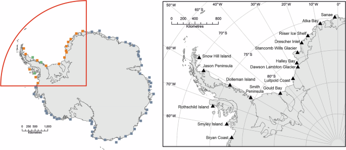
In the left panel orange squares show the 16 sites included in this study, green squares are sites with insufficient data, and grey squares represent the colonies outside our sector of interest. In the right panel, we identify the site names for the colonies included in this study.

Full size image

Satellite imagery

We used optical satellite data from the MAXAR VHR satellite constellation (https://resources.maxar.com/brochures/the-maxar-constellation) that was speculatively tasked over each colony location each year, accessed from the MAXAR search and Discovery platform (https://discover.maxar.com/ and similar previous versions). A single section of each image with a minimum window of 25 km² was obtained for each colony each year. In several cases, images were unsuitable as there was low cloud, low sun angle or poor environmental conditions obscuring or making penguins difficult to identify. Where possible, additional images were acquired. Additional information of image ID and scene quality is contained in Supplementary Table 5.

The analysis was restricted to the austral spring, between the end of August, when the sun comes up at the more northerly colonies, and the end of November before the adults depart the colonies as chicks fledge. The general method of pre-processing followed that of LaRue et al.³⁰, first loading each image into ArcGIS (ESRI ArcGIS version 10.6 2024 and earlier versions), and projecting the images into the local UTM projection for more accurate area assessment. Imagery was pan-sharpened using ArcGIS, and enhanced using a ‘Standard Deviation’ histogram stretch. The location of the colony was then isolated, and the colony was cropped from the surrounding image manually to avoid excessive processing time. A supervised classification analysis was then conducted on each image, using a multivariate classification analysis in ArcGIS, which involves training a model on manually chosen pixels of penguin, guano, snow and shadow. These training data were chosen manually by experienced observers and usually equated to between 50-200 examples from each class, depending upon the homogeneity of the background image. Once the classes have been identified the multivariate classification algorithm divides the image into the available classes, one of which will be penguins. This process is iterative and usually training data needs to be refined multiple times before an acceptable confidence (>95% agreement between manual and automated observations) is reached. From these results, the penguin pixels were isolated and converted into a shapefile. The shapefile gives the area occupied by penguins in each image. This process was undertaken for a total of 241 images over the 15-year period (see Supplementary Data 5).

Statistical analysis

To convert the area of penguins in each image to an index of abundance, we followed an approach similar to that used by LaRue et al. ³⁰, using a state-space analysis of emperor penguin population dynamics and observation process, and modified for satellite observations but without additional aerial or ground counts.

The population process accounted for daily changes in satellite counts over the survey period (August–November) in each of 16 identified colonies (Fig. 1). Colony-level trends and annual fluctuations were assessed considering the persistence of colonies at the same locations given physical changes (e.g. fast ice conditions), and occupancy (i.e. presence or absence for unknown reasons). The observation process accommodated bias and precision in satellite image counts due to data collection, and changes over survey period due to chick mortality and subsequent emigration by attendant and non-attendant adults.

Following LaRue et al. ³⁰, expected abundance at colony j and year y was (N_j,y=z_j,yX_j,y), where (X_j,y) and (z_j,y) are terms for abundance and a colony presence. The inter-annual change in colony abundance ((r_j)) was modelled as (X_j,y sim Lognormal(log (X_j,y-1)+r_j,sigma _pro^2)), where (sigma _pro^2) is the process variance. Due to a relatively low sample size and to the sparse data of some colonies, colony-level effects were modelled as random effects with (r_j sim Normalleft(barr,sigma _r^2right)).

As in most state-space population models³⁸, priors for initial population states ((X_j,1)) were given, and here we assumed a log-normal distribution with hyperparameters estimated empirically from the data as

Occupancy, or colony presence, was modelled with probability parameter p, as (z_j,y sim Bernoullileft(pright)). Although it was desired³⁰, due to a low sample of years with colony absences, occupancy was not modelled accounting for detectability, and variation due to colony or previous occupancy (autocorrelation) effects.

The observation process assumed that the size of the areas occupied by penguins in satellite images ((N_j,y)) were normally distributed, centred on the expected number of penguins present in the colony on the day of the survey ((D_j,i,y)), and corrected for an estimated bias (beta _i) in interpretation of satellite images; (N_j,yexp (alpha D_j,i,y)beta _i). As the number of adults declines over the spring survey period, we used a log-linear fixed effect ((alpha)) of (D_j,i,y), which was the calculated day of the year corresponding to survey date and subtracting the average mid-point of the annual surveys (day 300). (alpha) thus described the proportional change in expected count for each day elapsed in the survey³⁰.

Satellite counts were mapped to colony abundance as (S_j,i,y sim normal(N_j,yexp (alpha D_j,i,y)beta _i,w_j,y^2)), where (w_j,y^2=[(N_j,yexp (alpha D_j,i,y)beta _i)CV_S]^2). The variance term (w_j,y^2) assumed a constant coefficient of variation ((CV_S)), to be estimated when fitting the model, and assumed an increasing, but proportional, absolute error with colony size, which is common in image counts. Thus, separate fixed effects for (CV_S) and (beta _i) were estimated for each image quality score, which was arbitrarily assigned as poor (1), moderate (2) or good (3). These scores were related to the observers’ subjective ability to identify penguins in an image (similarly rated between 1 and 3), and to measured values of spectral band count, resolution, sun elevation, cloud cover, off nadir angle, collected GSD (ground sampling distance), and product GSD.

To accommodate observer bias, image quality scores were related to these variables in a discriminant analysis of principal components³⁹, using R package adegenet⁴⁰. Here, we selected the optimum number of principal components using cross-validation and used observer-assigned image quality as grouping variable in a discriminant analysis. The results provided a covariate with predicted image quality, and the subsequently fitted β coefficients assumed that satellite observations had a constant proportional bias.

Model fitting and assessment

We used Markov Chain Monte Carlo methods in program JAGS⁴¹, run from R (v.4.4.0; R Core Team, 2024)⁴² using package jagsUI⁴³ to fit the state-space models. We used 550,000 iterations of three Markov chains using dispersed parameter values as starting values and discarded the first 50,000 samples of each chain as burn-in, thinning the remainder to every 50th sample, which produced 10,000 posterior samples from each Markov chain. We assessed chain convergence visually using trace plots, through the mixing of the chains and sample autocorrelation plots and using the (widehatR) potential scale reduction factor statistic⁴⁴. We selected similar prior distributions as LaRue et al.³⁰ (Supplementary Tables 1–3), and we assessed the model’s goodness-of-fit using posterior predictive checks. We obtained the root mean square error of simulated data and the observed data and obtained and estimated Bayesian p-value. P-values close to 0.5 indicated a reasonable fit and occurred when the fitted statistical model was equivalent to the ‘true’ model, which generated the data (Supplementary Fig. S1).

Colony specific and general results can be seen in Fig. 2 and Supplementary Data 1–4.

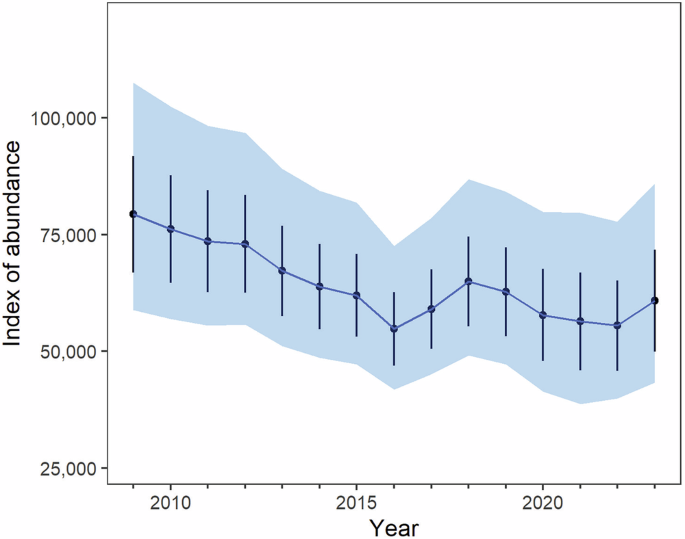
The blue area represents the 95% credible intervals and the solid value line the median of the posterior distribution simulations (in practical terms, these are the 0.025 and 0.975 percentiles of the posterior distribution of the abundance estimates). Black error bars are the mean estimates (or point estimates) of the abundance index plus and minus 1 standard error. The thicker blue line is the most likely scenario.

Full size image

Estimates for model parameters describing the emperor penguin population dynamics are in Supplementary Table S1. All the (widehatR) values were lower than 1.1, and together with their trace plots suggested a successful convergence. Of the datasets simulated for posterior predictive checks, 24% had satellite counts with lower root mean square error (RMSE) than the observed data (Bayesian p-value = 0.24), suggesting a reasonable fit (Supplementary Fig. S1).

In the entire study area between 2009 and 2023 there was a 0.94 probability of emperor penguin population decline; a 0.30 probability of a 30% decline; and a 0.005 probability of a 50% decline. This corresponds to a likely mean decrease of −22% (95% CI: −44.6 to +8.34%) (Fig. 2), equivalent to approximately −18,275 fewer adults in 2023 (95% CI: −42415 to 5844) than in 2009.

The population trajectory (log-linear annual rate of change) was −2.25% per year (−4.33% to +0.04%), and an estimated abundance index of 59,400 (95% CI: 43,424–86,200) of penguin area in late spring, without an unknown quantity of pre-breeders, failed breeders, and non-breeders. The probability of a 30% decline over three emperor penguin generations (16 years on average) was estimated as 0.91.

Regional trends are summarised in Fig. 3, Table S2 and percent population change over the study period in Table S3. All of the regions except the Antarctic Peninsula showed a decline over the period of the study. Although the estimates of long-term abundance shown were highly variable, the brevity of the study period limited the ability to detect significant trends.

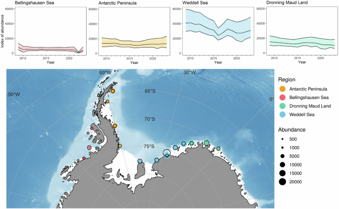
On the map, the size of the solid coloured circles denotes the relative size of the colony in 2023, the black outlines represent the size in 2009.

Full size image

Accuracy of the method

A primary concern when monitoring emperor penguins using VHR satellite imagery is the accuracy of the classification method. Uncertainty comes from two sources: (1) the errors associated with classifying the area of penguins as a metric of population; and (2) the potential variation in the population in late spring when the imagery is acquired^45,46 The levels of variability from each of these two sources are potentially important⁴⁵. With respect to the first issue, LaRue et al.³⁰ and this study use images linked to Bayesian statistics to produce an overall population trend. Bayesian statistics are based on the concept that probability is a measure of belief in an event and gives confidence values based upon not just the overall probability, but the amount of data used to calculate those statistics (La Rue et al. analysed 460 images³⁰, here we use 241). The population trend for both the LaRue et al.³⁰ and our analysis is based upon methods that have been developed and refined by different groups over many years. The common practices that have evolved are considered robust and best practice for the data available. With respect to the second issue, it is important to recognise that the timing of image acquisition in late spring, dictates that only a proportion of the adult population is in attendance at each colony, with an unknown proportion at sea foraging, or having already failed in their breeding attempt. As such, it is uncertain whether the area classified as penguins in the images reflects a true population estimate. However, recent work at Atka Bay suggests that adult attendance remains stable throughout spring, extending into late November or early December⁴⁶, so the estimate of population in spring is plausibly based upon a constant demographic component. Further, the image acquisition date is used as a parameter in the model to reflect this.

Previous work^24,30 has converted the index of area representing penguins into a number of penguin pairs, using aerial survey observation to ground truth satellite imagery; effectively equating one square metre to a single penguin based on a linear regression of the relationship between satellite derived area and actual counts from aerial survey²⁴, or via a parameter in the Bayesian model³⁰. These population estimates then reflect spring adult attendance at the colony, rather than a full breeding population estimate. In our analysis we are concerned with relative change, rather than population size per sea. Thus, we remove this potential source of error by reporting only the area of penguins as an index of abundance.

Interpretation of results

Our results build on those of LaRue et al.³⁰ and show an evident decline in population numbers in our sector of interest; this study suggests a decline in emperor penguin populations with a best fit of −22% over the 15 year period, equivalent to an absolute decline of 1.6 % per year (N15 = (100 − 22) × N0 = λ¹⁵ × N0, which gives λ = 0.984, meaning an annual decline of ca. 1.6%) or a log-linear annual rate of change of −2.25% per year. We report this decline with a very high probability (0.91 for a 30% decline over three generations (a total of 48 years as each generation is 16 years on average; cf 16.4 years reported by Bird et al.⁴⁷). Our results indicate a steep decline in population until 2016, followed by an undulating plateau in population size after that point. Although the 15-period of our study is relatively short for a long-lived species, it does approximately represent one breeding lifetime of the emperor penguin, which on average lives 20 years and first breeds at around 5 years of age. As indicated above, successful annual breeding for this species is more critical than most other birds and skipping breeding in poorer years is not a long-term option. Therefore, the relatively short time series shown here is important and highly relevant to our study that it might be for many other avian species.

Our analyses reflect a quarter of the Antarctic coastline and, as such, may not be representative of the whole continent. Environmental conditions and patterns of sea-ice extent are regional (Fig. 4). Our sector of interest has been subject to a greater decline in sea-ice extent, especially in the Bellingshausen Sea region.

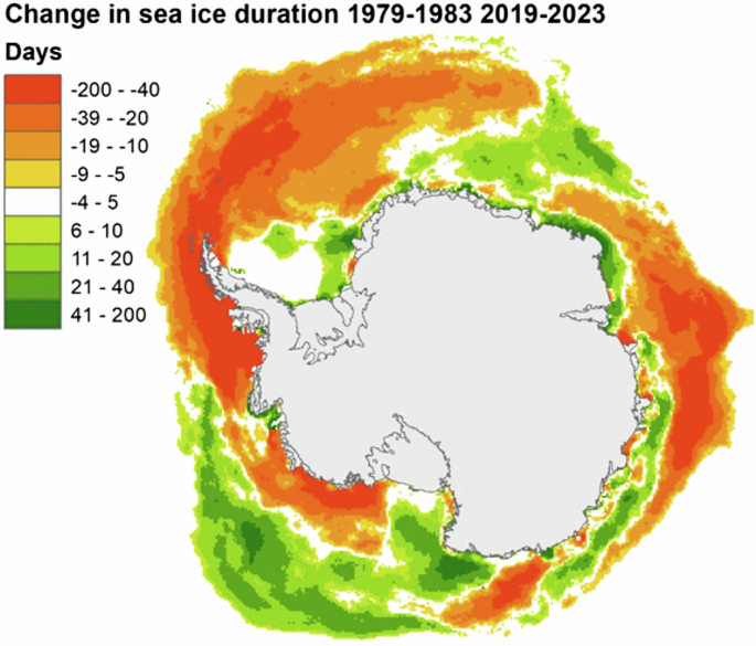
Change in sea ice duration (in days per year) around Antarctica (Sea Ice Index dataset: https://nsidc.org/data/g02135/versions/3 accessed 01/08/2024.

Full size image

Interestingly, although the sea-ice duration in the Bellingshausen Sea sector has reduced significantly (Fig. 5A), the decrease in our emperor penguin index for this region has not tracked sea-ice decline. This is in marked contrast to the Weddell Sea (Fig. 5B), where sea-ice duration has been variable³¹, but the decline in our emperor penguin index has been significant. In the Bellingshausen Sea region, sea-ice loss in 2022 was extensive and three of the four colonies analysed in the region in this study had no adults present³³. It is plausible that breeding was initiated at these colonies, but breeding failure subsequently occurred. When the sea ice returned in 2023, numbers were lower than average.

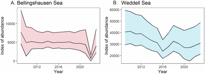
A Bellingshausen Sea regional index of abundance (based on x colonies) showing the extreme event in 2022. B Weddell Sea regional index of abundance (based on y colonies). The loss of the Halley Bay colony in 2016 is evident, followed by a slight upturn as adults relocated to the Dawson-Lambton colony.

Full size image

In the Weddell Sea, the collapse of the Halley Bay colony in 2016³⁴ is a major factor. This colony was originally one of the largest in Antarctica but suffered breeding failures in each year subsequently. After the sea ice break-up in 2016, most of the adult population emigrated to the Dawson Lambton colony, 85 km to the south, where sea ice conditions remained stable. Taken together, the Halley Bay and Dawson Lambton index of abundance showed that the adult population had recovered by 2018 (see Supplementary Fig. 2). The loss of production between 2016 and 2018 is likely to have been significant and may account for a degree of inter-annual variation in the Weddell Sea combined index. Importantly, however, the combined index for the two colonies shows a decline prior to 2016, with an abundance index of ~20,000 in 2010 and ~12,000 in 2015 (Supplementary Figs. 1 and 2). The underlying cause of this decline before 2016 remains unclear.

Comparison with the published results from LaRue et al.³⁰ (see Supplementary Fig. 3), on a regional and overall level, shows good correspondence between 2009 and 2015, with each year’s combined overall value within 7% of each other. However, in the years 2016–2018 our estimates are lower than the LaRue estimates of the same colonies (by 18.6%, 20.4% and 17.8% respectively, see Supplementary Data 6). In 2016 and 2017, this can be partially explained by a slight difference in methodology, specifically of treatment of the zero count at Halley Bay due to early sea ice loss in these years. In our analysis, colonies that have no penguins in the imagery are counted as zero, reflecting the abundance at the time, but in the LaRue et al.³⁰ analysis they are classed as null on the assumption that a breeding population was at the site in the winter before the image was taken in the spring. This can be seen as a difference between our aim to estimate relative springtime abundance, rather than provide an absolute population estimate at each site in each year. However, this reasoning does not fully explain all of the discrepancy in 2016, 2017 and 2018. In these years, lower estimates at three sites: Atka Bay, Gould Bay and Smyley Island are responsible for 88% difference, with the largest difference at Smyley Island (44% of the total difference). Most colonies, however, still show similar estimates in these years. Why these three colonies exhibited very different results is difficult to assess, but it does highlight the high potential variance of estimating emperor population at individual colonies using this methodology.

Why have emperor penguin populations declined?

Attributing a reason why emperor penguin numbers have declined in this sector is complex and, as yet, poorly understood. Previous work has shown that population numbers are affected by fast ice extent, with low fast ice leading to early ice break-out and poor breeding success and excessive fast ice extent leading to higher rates of adult mortality^5,48,49. Reduced sea ice extent and early ice-breakout since 2016 have been noted in several areas, but the majority of the population decline shown in this paper has been in the period between 2009 and 2015, before the well documented years of extreme low sea ice that have been observed recently^7,8. It must follow, therefore that other environmental factors are the main drivers of population decrease in this sector.

One colony, located within this sector but not included in this study, is the site on the Dion Islands that is likely to be functionally extinct. This colony decreased in population almost continually from the late 1970s until 2009, when no breeding birds were recorded³⁷. Since its discovery in the 1940’s the small colony was located on an island, so breeding success due to lack of sea ice as a breeding platform could not have been a major factor, and other drivers must have reduced the population. The location, in Marguerite Bay on the West Antarctic Peninsula has witnessed rapid warming over the last 50 years^50,51 and the Trathan et al. ³⁷ study lists some of the implications of this warming as potential drivers of change. They include reduced prey availability as pack-ice conditions change and oceans warm; increased competition from other predators as they move into the area to exploit the marine resources; lack of fresh snow at the site that emperors use to re-hydrate while breeding; and increased disturbance and predation as other predators move into the area with the warmer conditions and more open ocean environment. It is likely that these factors may now be affecting several of the other emperor colonies in this sector.

The other ice-obligate penguin species, the Adélie (Pygoscelis adeliae), has been shown to have adapted its foraging strategy when sea ice cover is low. In times of no or little sea ice, adults must dive deeper to catch prey, which takes more effort and lowers breeding success^52,53. Conversely, and much like earlier studies on emperor penguins, excessive sea ice cover can also be detrimental as adults need to walk further across the ice to access foraging grounds. Recent work has also shown that juvenile emperor penguins exhibit very high interannual variability in body mass, which has important impacts on juvenile survival, and which is tightly associated with sea ice extent during the chick-rearing period¹².

There are also other potential drivers linked to rainfall and storminess. Studies on Adélie penguins have shown that increased storms and extreme rainfall can seriously impact breeding success^54,55. Extreme storms and precipitation events result in flooding of nests, which drenches chick,s necessitating the use of more energy to regulate temperature. Although nest flooding is not a problem for emperors, personal observations (PTF) support this hypothesis that chick drenching can contribute to mortality as an unusually early extreme rainfall event in mid-October was observed causing the death of several hundred otherwise healthy chicks at the Snow Hill Island colony in 2010. The Antarctic Peninsula has already seen increased storminess, snowfall and rainfall⁵⁶ and it is likely that, for more northerly or warmer colonies, increased and earlier rainfall events around the coast could be a driver of population change. Other potential causes of chick wetting linked to warming temperatures, such extensive melt pools on the surface of the sea ice in warm years, could also have detrimental effects on breeding success. Analogous to the situation for Adélie chicks, these pools can lead to chick wetting and increased energy expenditure, but like all of these environmental factors, these potential drivers have not yet been quantified for emperor penguins.

A final consideration is huddle size⁵⁷. As colony size decreases, the huddling ability of emperors in winter or during spring storms becomes less effective. As extreme events are predicted to increase and colonies decrease in size, a smaller huddle size may lead to failed incubation and poor body condition in over-wintering adults.

If we are to understand the drivers of emperor penguin populations and more effectively project their future status it is essential that studies on various potential drivers linked to warming temperatures are implemented. However, what is clear is that emperor penguin populations are already in decline.

The decline of the emperor penguin population in our sector of interest demonstrates a clear negative trend. Although there is significant variance in the model, the best fit results suggest a 22% decline over the 15-year period, something that is much greater than the rate of decline predicted by the process-oriented metapopulation demographic models based on high emission IPCC climate change scenarios (e.g.¹) (Fig. 6).

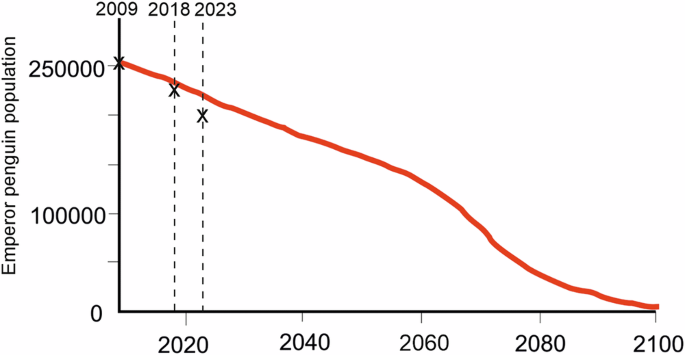
The first X on the left marks the initial global population estimate (Trathan et al.²) of 256,000 breeding pairs, the second denotes the estimated global decline of 9.5% reported by LaRue et al.³⁰ and the third is (best fit) decline of 22% reported in this paper, albeit expanded from a sectorial scale analysis; comparing the results from this regional assessment to the modelled global projection.

Full size image

Our results support the findings of LaRue et al.³⁰; however, we also show that populations in our sector of study continued to decline after 2018. Our overall results indicate a 91% probability of a 30% decline in the adult population in the study area over three generations (~48 years). Should this trend be reflected at a circumpolar scale, it suggests that emperor penguins should be classified on the IUCN Red List at “Vulnerableâ€�. Such a change would facilitate designation by the ATCM as an Antarctic Specially Protected Species. We recommend that comparable analyses are now undertaken for other parts of the Antarctic continent.